Sample Exam Problems
Click here for data and code files necessary to complete the practice problems.
-
The provided text file (
readings.txt) contains a timestamp broken up into year, month, day, hour, minute, second, and timezone components, as well as a reading from a sensor. Write a script that reads the data from the file into MATLAB.The script must:
- Place the timestamps in a single array of type
datetimestored in a variable named dates. Using the timezone component is optional. - Place numeric values for the readings in a single array of type
doublewith a variable name ofreadings.
- Place the timestamps in a single array of type
-
The provided data file (
viewdata.mat) contains a 19-by-3 matrixviewdatawith the following columns:- VideoLength: Length in minutes for the video
- Views: Number of times the video has been viewed
- MinutesWatched: Total amount of time viewers spent watching the video
Write a MATLAB script to analyze the data to determine the effect of video length on viewer retention with the following steps:
- Load the saved viewership data into the MATLAB workspace.
- Create a table column
PercentViewedcontaining the percentage viewed for each video according to the following formula: Percentage viewed = (Minutes watched / Views) / (Video length). - Create a table column
VideoTypethat identifies whether a video is short (Video length < 1.5), medium (1.5 <= Video length <= 2.25), or long (Video length > 2.25). - Use these new columns in
viewdatato calculate the mean percentage viewed for each video type. Store the results in a separate table. The new table should have three rows and two columns. One column should have the video type (short, medium, long) and one column should have the mean percentage viewed.
-
The provided data file (
TData.mat) contains temperature data reported by weather stations at the same instance in time. The contents of the data file are:- The x-coordinates of the weather station locations (in km) stored in the column vector
x - The y-coordinates of the weather station locations (in km) stored in the column vector
y - The temperature data corresponding to the station locations (in degrees C) stored in the column vector
T
Write a MATLAB script to load the data from the file and produce a contour plot similar to the one below with the temperature stations. Use the griddata function with '
v4' as the interpolation method to estimate the temperatures for the x-y spatial grid points.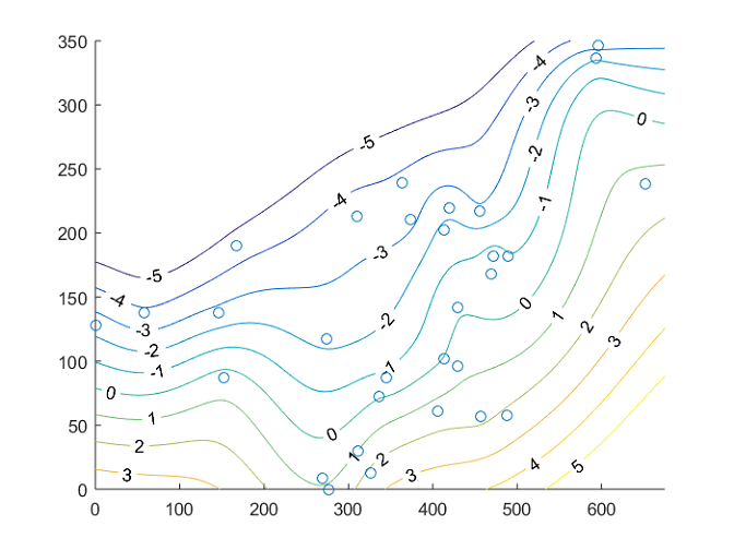
The plot must contain:
- contours spanning –5 degrees C to 5 degrees C in 1-degree increments
- a spatial extent of the contour plot corresponding to 0 < x < 675, 0 < y < 350, with a grid resolution (grid square size) of 1 km-by-1 km
- labels for each contour
- markers for the weather station locations
- The x-coordinates of the weather station locations (in km) stored in the column vector
-
Create an anonymous function
fthat accepts a (possibly vector valued) numeric input and returns a (possibly vector valued) numeric output according to the mathematical formula f(x) = x^2 – sin(x). Use this function along with thefminsearchfunction to find the local minimum value near the initial value nearx0 = 0.5.Store the local minimizing value and the corresponding function value in the variablesxminandymin, respectively.
-
A function called
viewImageaccepts an image and a variable number of parameter name/value pairs as shown in the following examples:viewImage(I,"zoom",2.3)
viewImage(I,"rotate",-15,"zoom",1.4)
viewImage(I,"adjust","dark")In the provided function, add code to the function body that validates the input arguments. The use of an arguments block is recommended. The function should produce an appropriate error message if any of the following conditions on the input arguments are not met:
- The input
Imust always be present and a numeric variable. - The optional inputs must be name/value pairs, where the names are one of the following: "
zoom,""rotate,"or "adjust." - The value following the names
"zoom"and"rotate"must be numeric scalars. - The value following
"adjust"must be a string with a value of"bright"or"dark."
Do not write any implementation beyond the code required to perform the validation.
- The input
-
The provided script
(diceSimulation.m)runs a simulation of rolling six, 6-sided dice and calculating the sum. The simulation is repeated 1,000,000 times to create a histogram of the probability distribution as shown below.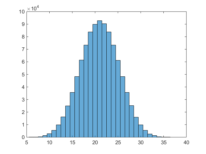
The code produces the correct result, but can be improved to run faster. Rewrite the script such that the simulation runs faster than the original. The updated script must produce the same results with 1,000,000 trials and display a histogram.
The figure illustrates one result from running the script. Solutions should have a similar distribution.
-
The provided script
(LoadData.m)loads data from an impact simulation and uses theyyaxiscommands to plot position on the left y-axis and velocity on the right y-axis. Modify the script to make the figure look as shown in the figure below.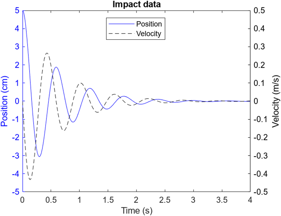
The figure must contain:
- an x-axis with a minimum value of 0 and a maximum value of 4
- a plot of the position vector as a solid blue line
- a left y-axis colored in blue with a minimum value of –5 and a maximum value of 5
- a plot of the velocity vector as a dashed black line
- a right y-axis colored in black with a minimum value of –0.5 and a maximum value of 0.5
- a title reading "Impact data" as shown in the figure
- a legend in the top center of the axes with the correct label for each plot
-
The provided app (see screenshot below) plots a sine wave based on the provided amplitude and frequency using the equation
y = amplitude*sin(2*pi*frequency*x)on the interval defined by[0 1].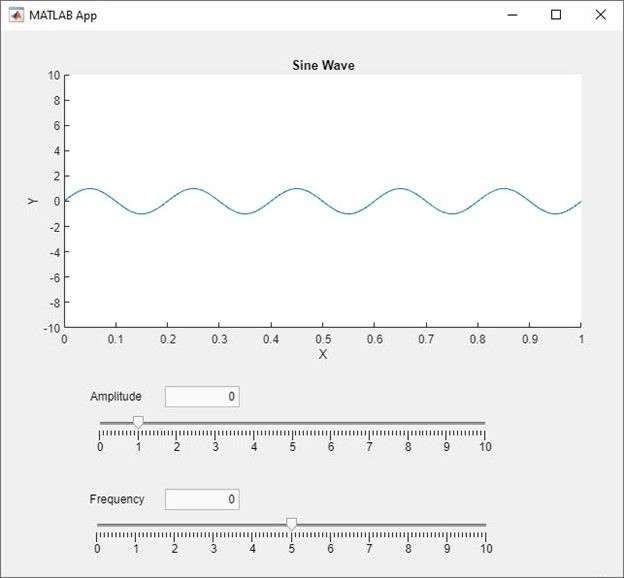
Write the callback functions for the slider controls to update the plot. The callbacks must:
- Update the plot with the new amplitude or frequency.
- Update the display of the amplitude and frequency values
app.AmplitudeEditFieldandapp.FrequencyEditField, respectively.
Additionally, display a plot with the default values for amplitude and frequency upon starting the app.
You can also select a web site from the following list
Americas
- América Latina (Español)
- Canada (English)
- United States (English)
Europe
- Belgium (English)
- Denmark (English)
- Deutschland (Deutsch)
- España (Español)
- Finland (English)
- France (Français)
- Ireland (English)
- Italia (Italiano)
- Luxembourg (English)
- Netherlands (English)
- Norway (English)
- Österreich (Deutsch)
- Portugal (English)
- Sweden (English)
- Switzerland
- United Kingdom (English)
Asia Pacific
- Australia (English)
- India (English)
- New Zealand (English)
- 中国
- 日本Japanese (日本語)
- 한국Korean (한국어)