What Is Stereo Reconstruction?

Stereo reconstruction estimates the depth of a scene by comparing two images captured from slightly different viewpoints, such as from two cameras, separated by a known distance T (the baseline) and sharing a focal length f, observing the same scene from different angles. As a result, the projection of a single 3-D point appears at different pixel locations in each image, producing a measurable difference, referred to as disparity. Given the known camera geometry, you can convert this disparity into depth, enabling you to reconstruct the 3-D structure of a scene using a stereo reconstruction framework.

How Does Stereo Reconstruction Work?

Stereo reconstruction relies on identifying corresponding pixels between the left and right images of a stereo camera system. Once you find a matching pair, you can compute the 3-D positions of points in a scene using triangulation.

Conceptually, this process consists of projecting rays from each camera center through the corresponding image points. The intersection of these rays in space determines the 3-D location of the point. Repeating this process for many pixels produces a 3-D representation of the scene, often in the form of a point cloud.

This figure illustrates a 3-D point P projected into two camera views, resulting in the image points (x₁, y₁) and (x₂, y₂) on the respective image planes, and the triangle formed by the line from each camera to its projection point and the baseline distance T between the cameras.

Once you have identified corresponding pixels in the left and right camera images, you can use the geometry of the stereo camera setup to calculate the depth of each point. To compute the depth Z of a point P, use the similarity of the triangle formed by the two cameras and P:

$Z = \frac{f T}{d}$

where d = x₁ — x₂, is the disparity, defined as the difference in the horizontal position between the two views. This means that points closer to the cameras have larger disparities, while points further away have smaller disparities. For example, an object close to the cameras appears at significantly different positions in the two images, creating a large shift. In contrast, distant objects appear at nearly the same position in both images, resulting in a small disparity. Thus, depth estimation reduces to measuring the disparity between matching pixels.

3-D Reconstruction Framework

The 3-D reconstruction framework consists of a sequence of key stages that transform stereo image pairs into accurate depth information.

Stereo Camera Calibration

Before you can accurately compute depth, you must calibrate the stereo camera system. Calibration determines the intrinsic parameters (focal length, principal point, and lens distortion) of each camera and their extrinsic relationship (relative position and orientation). You typically perform calibration using multiple images of a known pattern, such as a checkerboard.

This step ensures that:

Lens distortions are corrected.
Images can be rectified so corresponding points lie on the same rows.
Disparities can be accurately converted to real-world distances.

Epipolar Geometry and Camera Rectification

Use epipolar geometry to determine the relationships between points in the two images. This geometry describes how a 3-D point projects onto both image planes. For any point in the first image, the corresponding point in the second image must lie along a specific line called the epipolar line.

Aligned Cameras — When two cameras are perfectly aligned, with parallel optical axes and coplanar image planes, corresponding points in the left and right images appear on the same horizontal row. With this configuration, corresponding points need only be searched for along image rows. The disparity between these points directly relates to the depth of the corresponding scene point.
Unaligned Cameras — Not all stereo camera systems are perfectly aligned. In many practical situations, the cameras might be positioned at different angles or heights, which makes it more challenging to find which pixels in the two images correspond to the same 3-D point. In these cases, the relationship between points in the left and right images is different. A point in one image could correspond to a point anywhere along a line in the other image, rather than just along the same row.
Because epipolar geometry describes the geometric relationship between corresponding points using the epipolar line as a constraint, it reduces the search for correspondences from the entire image to just along the epipolar line. This makes the matching process more manageable, even when the cameras are not aligned. This figure illustrates a general stereo camera setup, showing how a point in the first image, p₁ of Camera 1, lies on a specific epipolar line of Camera 2.

Rectification for Simplified Disparity Estimation

When cameras are not aligned, epipolar lines can appear at arbitrary orientations, making it difficult to identify corresponding points between images. Rectification uses epipolar geometry to transform the images so that their epipolar lines become horizontal and aligned with the image rows.

After rectification, corresponding points lie on the same row in both images, reducing the correspondence problem to a one-dimensional search along each row. This simplification makes stereo matching more efficient and reliable.

Convert Disparity to Depth

After rectification, corresponding points between the two aligned images lie on the same row. For each pixel in the left image, the corresponding pixel in the right image appears along that same row, but generally at a different column position. The disparity is the difference between the column positions of these corresponding points. In other words, disparity measures how much a point has shifted left or right between the two images.

Once you know the disparity for each point, you can use it to compute the depth of that point in the scene. Given the camera focal length f and the baseline T, defined as the distance between the optical centers of the two cameras, you can recover depth using the standard geometric relationship:

$Z = \frac{f T}{d}$

where Z is the depth and d is the disparity. Applying this relationship across all image points produces a depth map or a 3-D point cloud, representing the three-dimensional structure of the scene.

Implement 3-D Stereo Reconstruction Framework Using Computer Vision Toolbox

Stereo reconstruction using Computer Vision Toolbox™ involves these steps, each of which shows the purpose, key functions, and outputs involved in obtaining a dense 3-D reconstruction from a stereo camera pair.

Stereo Camera Calibration
Calibrate the two-camera system to determine the intrinsic parameters of each camera and the extrinsic transformation between them. Use the Stereo Camera Calibrator app or the estimateCameraParameters function with multiple pairs of calibration pattern images.
Calibration produces a stereoParameters object, which contains the intrinsic parameters of each camera and the extrinsic transformation between them. You can use this object for image rectification and converting disparities to real-world distances. Calibration accuracy depends on camera resolution and baseline length. Choose a baseline so that objects at the farthest expected distance still produce a measurable disparity. To verify the estimated camera poses and extrinsic parameters, use the showExtrinsics function.
Stereo Image Rectification
Rectify the stereo images so that corresponding points lie on the same image rows.
For calibrated stereo cameras, use the rectifyStereoImages function with the stereoParameters object obtained from calibration. For uncalibrated cameras, estimate projective transforms for each image using estimateStereoRectification, then pass the resulting transforms to rectifyStereoImages. This approach does not require camera intrinsic or extrinsic parameters.
The rectifyStereoImages function returns the rectified left and right images, along with a reprojection matrix, used to convert disparity values into 3-D coordinates.
You can visualize the rectified image pairs using the stereoAnaglyph function to verify that corresponding features are properly aligned along the same row. For additional information about rectifying uncalibrated stereo images, see Uncalibrated Stereo Image Rectification.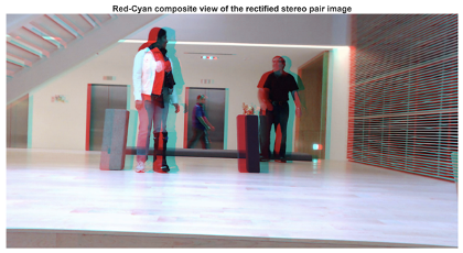
Disparity Map Computation
Compute the horizontal shift (disparity) between corresponding pixels in the rectified stereo images. In rectified images, you measure disparity along image rows. Closer objects have a larger disparity, while objects further away have a smaller disparity, reflecting the inverse relationship between disparity and depth.
You can produce a disparity map as an image where each pixel value represents the horizontal shift (in pixels) of that point between the left and right images. To compute dense disparity maps , use the disparityBM (block matching) or disparitySGM (semi-global matching) function. The disparitySGM function generally produces smoother and more accurate results.
Disparity estimation can be challenging in regions with little texture, such as smooth walls or sky, because pixel matches are ambiguous along those rows. In such scenarios, deep learning–based methods, such as the opticalFlowRAFT object that implements the recurrent all-pairs field transform (RAFT) algorithm, can improve accuracy. For more information, see Compare RAFT Optical Flow and Semi-Global Matching for Stereo Reconstruction.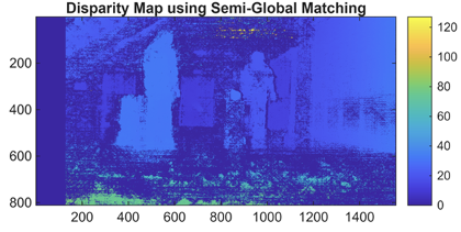
Dense 3-D Reconstruction
Convert the disparity map into real-world 3-D coordinates using the stereo camera geometry determined during calibration and rectification. This known geometry includes the camera baseline, focal length, and the reprojection matrix obtained from the rectification step.
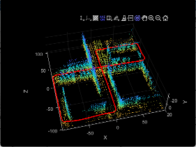
This process, called depth-from-disparity, reprojects each disparity value into 3-D space, producing a dense 3-D representation of the scene. To perform this operation, you can use the reconstructScene function with the disparity map and the reprojection matrix. The function returns an array of xyz-coordinates for each pixel in the coordinate system of the reference camera (Camera 1), forming a dense 3-D point cloud.
The resulting point cloud captures the three-dimensional structure of the scene, and you can use it for visualization, distance measurement, or further 3-D processing. You can visualize the point cloud using the pcshow function, or convert the data to a pointCloud object for additional operations, such as filtering, outlier removal, or color mapping, enabling interactive exploration and analysis.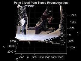

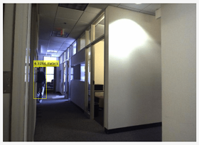
Applications of Stereo Reconstruction

Stereo reconstruction is used in a wide range of computer vision and robotics applications that require depth perception or understanding of 3-D environments. This table lists some common use cases and provides examples illustrating how to apply stereo reconstruction in each context.

Application	Examples	Visualization
Distance estimation, obstacle detection, and navigation	Depth Estimation from Stereo Video Measure Real-World Distances to Objects Using a Stereo-Camera
3-D mapping and SLAM with scale estimation	Stereo Visual SLAM for UAV Navigation in 3D Simulation Performant and Deployable Stereo Visual SLAM with Fisheye Images Stereo Visual Simultaneous Localization and Mapping
3-D scene reconstruction and measurement	Reconstruct 3-D Scene from Stereo Image Pair Using Semi-Global Matching Compare RAFT Optical Flow and Semi-Global Matching for Stereo Reconstruction

Application

Examples

Visualization

Distance estimation, obstacle detection, and navigation

Camera image with distance measurement to an object in the image.

3-D mapping and SLAM with scale estimation

Map and camera trajectory generated using stereo visual SLAM.

3-D scene reconstruction and measurement

Colored 3-D point cloud obtained from stereo reconstruction.

References

[1] Torralba, Antonio, Phillip Isola, and William T. Freeman. Foundations of Computer Vision. Adaptive Computation and Machine Learning Series. The MIT Press, 2024.

[2] Hartley, Richard, and Andrew Zisserman. Multiple View Geometry in Computer Vision. 2nd ed. Cambridge University Press, 2004. https://doi.org/10.1017/CBO9780511811685.

[3] Faugeras, Olivier. Three-Dimensional Computer Vision: A Geometric Viewpoint. Repr. Artificial Intelligence. MIT Press, 1993.

[4] Hirschmuller, H. Accurate and Efficient Stereo Processing by Semi-Global Matching and Mutual Information. 2005 IEEE Computer Society Conference on Computer Vision and Pattern Recognition (CVPR’05) 2 (2005): 807–14. https://doi.org/10.1109/CVPR.2005.56.