bernsteinMatrix

Bernstein matrix

Syntax

B = bernsteinMatrix(n,t)

Description

B = bernsteinMatrix(n,t), where t is a vector, returns the length(t)-by-(n+1) Bernstein matrix B, such that B(i,k+1)= nchoosek(n,k)*t(i)^k*(1-t(i))^(n-k). Here, the index i runs from 1 to length(t), and the index k runs from 0 to n.

The Bernstein matrix is also called the Bezier matrix.

Use Bernstein matrices to construct Bezier curves:

bezierCurve = bernsteinMatrix(n, t)*P

Here, the n+1 rows of the matrix P specify the control points of the Bezier curve. For example, to construct the second-order 3-D Bezier curve, specify the control points as:

P = [p0x, p0y, p0z;  p1x, p1y, p1z;  p2x, p2y, p2z]

Examples

2-D Bezier Curve

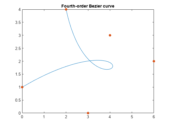
Plot the fourth-order Bezier curve specified by the control points p0 = [0 1], p1 = [4 3], p2 = [6 2], p3 = [3 0], p4 = [2 4]. Create a matrix with each row representing a control point.

P = [0 1; 4 3; 6 2; 3 0; 2 4];

Compute the fourth-order Bernstein matrix B.

syms t
B = bernsteinMatrix(4,t);

Construct the Bezier curve.

bezierCurve = simplify(B*P);

Plot the curve adding the control points to the plot.

fplot(bezierCurve(1), bezierCurve(2), [0, 1])
hold on
scatter(P(:,1), P(:,2),'filled')
title('Fourth-order Bezier curve')
hold off

3-D Bezier Curve

Construct the third-order Bezier curve specified by the 4-by-3 matrix P of control points. Each control point corresponds to a row of the matrix P.

P = [0 0 0; 2 2 2; 2 -1 1; 6 1 3];

Compute the third-order Bernstein matrix.

syms t
B = bernsteinMatrix(3,t);

Construct the Bezier curve.

bezierCurve = simplify(B*P);

Plot the curve adding the control points to the plot.

fplot3(bezierCurve(1), bezierCurve(2), bezierCurve(3), [0, 1])
hold on
scatter3(P(:,1), P(:,2), P(:,3),'filled')
hold off

3-D Bezier Curve with the Evaluation Point Specified as a Vector

Construct the third-order Bezier curve with the evaluation point specified by the following 1-by-101 vector t.

t = 0:1/100:1;

Compute the third-order 101-by-4 Bernstein matrix and specify the control points.

B = bernsteinMatrix(3,t);
P = [0 0 0; 2 2 2; 2 -1 1; 6 1 3];

Construct and plot the Bezier curve. Add grid lines and control points to the plot.

bezierCurve = B*P;
plot3(bezierCurve(:,1), bezierCurve(:,2), bezierCurve(:,3))
hold on
grid
scatter3(P(:,1), P(:,2), P(:,3),'filled')
hold off

Input Arguments

n — Approximation order

nonnegative integer

Approximation order, specified as a nonnegative integer.

t — Evaluation point

number | vector | symbolic number | symbolic variable | symbolic expression | symbolic vector

Evaluation point, specified as a number, symbolic number, variable, expression, or vector.

Output Arguments

B — Bernstein matrix

matrix

Bernstein matrix, returned as a length(t)-by-n+1 matrix.

Version History

Introduced in R2013b