Autonomous Underwater Vehicle Pose Estimation Using Analytical Jacobians in Custom Sensor Models

This example uses:

This example shows how to estimate the pose of an autonomous underwater vehicle (AUV) by using analytical Jacobians in custom sensor models. In this example, you define and tune an extended Kalman filter to fuse noisy sensor data, and then estimate and visualize the vehicle trajectory. You also compare pose estimates with smoothed estimates and analyze corresponding position errors.

Define Problem Statement for AUV Pose Estimation

To estimate the position and orientation of an AUV, you use an extended Kalman filter (EKF) [1] to fuse a vehicle motion model with noisy sensor measurements. The EKF is the nonlinear counterpart of the Kalman filter [2]. The EKF represents uncertainty about the vehicle state with a normal (Gaussian) distribution described by two quantities: a mean $x$ of the current best estimate and a covariance matrix $P$ of the associated uncertainty. The state can include position $r$ , velocity $v$ , orientation $q$ , and other navigation variables.

In the "predict" or propagate step, a nonlinear dynamics model advances the vehicle state following the formula:

$\frac{d x}{d t} = f (x, u) + noise$ ,

where $u$ is the control input and $f$ is the state dynamics motion model. The EKF linearizes this model around the current estimate using the Jacobian $F = \partial f / \partial x$ to propagate the covariance matrix $P$ .

In the "correct" or update step, you compare measurements $z$ with the corresponding measurement model, which is evaluated using the current state estimate $h (x)$ . You compute the Kalman gain $K$ by using the linearized measurement model $H = \partial h / \partial x$ . To correct the state and reduce uncertainty, the Kalman gain weights the residual $z - h (x)$ . A typical discrete update step is:

${x_{}^{ˆ}}^{+} = {x_{}^{ˆ}}^{-} + K (z - h ({x_{}^{ˆ}}^{-}))$ ,

where ${x_{}^{ˆ}}^{-}$ is the predicted state (just prior to the update) and ${x_{}^{ˆ}}^{+}$ is the corrected state (just after the update). For this reason, accurate Jacobians $F$ and $H$ are crucial for stability, convergence, and computational efficiency.

When estimating the pose of a vehicle, such as a submarine, you can create custom motion and sensor models to use with the insEKF (Navigation Toolbox) object in Navigation Toolbox™. You create these models by using the base classes positioning.INSMotionModel and positioning.INSSensorModel. In these custom models, you can provide analytical measurement Jacobians to improve accuracy and efficiency of the pose estimation, instead of relying on default numerical differentiation.

To complement the built-in inertial measurement unit (IMU), magnetometer, GPS, and motion models, this example defines three custom positioning.INSSensorModel subclasses:

insDepth — A depth sensor model that measures the vehicle's down position (trivial identity Jacobian)
insSpeed — A flow‑relative speed sensor model that projects the vehicle’s fluid‑relative velocity onto the body x‑axis (nontrivial Jacobian with respect to orientation, velocity, and flow)
insZuptVyz — A two-axis "zero‑velocity update" (ZUPT) sensor model that expects body‑frame y and z velocities to be zero (nontrivial Jacobian with respect to orientation and velocity)

You provide the measurement Jacobian $H$ in these three custom sensor models for the EKF update step.

While this example enforces a two-axis ZUPT sensor model, you could add a custom motion model to directly enforce a "no side slip" constraint on the vehicle dynamics. In this case, you would provide the appropriate motion model Jacobian $F$ , which is used in the EKF predict step to propagate the state error covariance. Similarly, this approach can be extended to incorporate any other customizations you want to add to the motion model.

To compute Jacobians analytically, you can use Symbolic Math Toolbox™. In this example, you will symbolically derive expressions for the following quantities:

The navigation-to-body-frame transformation matrix from the quaternion
The body‑frame velocity transformed from the navigation‑frame (with and without fluid flow)
The corresponding measurement Jacobians needed by insSpeed and insZuptVyz

From these symbolic expressions, you generate code for MATLAB® functions. You can use these functions in custom classes without requiring Symbolic Math Toolbox at run time. You integrate the generated Jacobian functions (SpeedJacobian and ZuptVyzJacobian) into the custom sensor classes to provide analytic measurement Jacobians to insEKF.

With these models, you can simulate an AUV dive‑and‑surface trajectory. You fuse IMU, magnetometer, and GPS readings with depth, flow‑relative speed, and ZUPT measurements in the insEKF object. Finally, you evaluate estimation accuracy along the trajectory, and apply smoothing to further refine the pose estimates.

Derive Quaternion, Rotation Matrix, and Jacobians

Using Symbolic Math Toolbox, you can derive a rotation matrix from a quaternion, perform velocity transformations from the navigation frame to the body frame, and compute Jacobians of the velocity measurements.

Define Quaternion and Rotation Matrix

First, define a unit quaternion, which consists of a scalar part $q_{0}$ and a 3-by-1 vector part $q = {(q_{1}, q_{2}, q_{3})}^{T}$ .

syms q0 real
syms q [3 1] real
qSym = [q0; q]

qSym = 
 $(\begin{array}{c} q_{0} \\ q_{1} \\ q_{2} \\ q_{3} \end{array})$

To represent the cross product ${[\begin{array}{c} q \end{array}]}_{\times} = q \times$ , generate a skew-symmetric matrix for the vector part of the quaternion.

qskew = cross([q q q],eye(3))

qskew = 
 $(\begin{array}{ccc} 0 & - q_{3} & q_{2} \\ q_{3} & 0 & - q_{1} \\ - q_{2} & q_{1} & 0 \end{array})$

Compute the rotation matrix from the navigation frame to the body frame using this formula [3]:

$T_{nav}^{body} = {(q \otimes q + q_{0}^{2} I + 2 q_{0} {[\begin{array}{c} q \end{array}]}_{\times} + {[\begin{array}{c} q \end{array}]}_{\times}^{2})}^{T}$

Tn2bsyms = ((q*q') + q0^2*eye(3) + 2*q0*qskew + qskew^2)'

Tn2bsyms = 
 $(\begin{array}{ccc} {q_{0}}^{2} + {q_{1}}^{2} - {q_{2}}^{2} - {q_{3}}^{2} & 2 q_{0} q_{3} + 2 q_{1} q_{2} & 2 q_{1} q_{3} - 2 q_{0} q_{2} \\ 2 q_{1} q_{2} - 2 q_{0} q_{3} & {q_{0}}^{2} - {q_{1}}^{2} + {q_{2}}^{2} - {q_{3}}^{2} & 2 q_{0} q_{1} + 2 q_{2} q_{3} \\ 2 q_{0} q_{2} + 2 q_{1} q_{3} & 2 q_{2} q_{3} - 2 q_{0} q_{1} & {q_{0}}^{2} - {q_{1}}^{2} - {q_{2}}^{2} + {q_{3}}^{2} \end{array})$

Compute Jacobian for Flow-Relative Velocity in Body Frame

Next, define 3-by-1 symbolic vectors for the vehicle velocity in the navigation frame $v$ and the flow velocity $v_{flow}$ .

syms v v_flow [3 1] real

To calculate the flow-relative velocity of the vehicle, transform the vehicle velocity from the navigation frame to the body frame using this formula:

$h = T_{nav}^{body} (v - v_{flow})$

vb = Tn2bsyms*(v - v_flow)

vb = 
 $(\begin{array}{c} (v_{1} - v_{flow1}) ({q_{0}}^{2} + {q_{1}}^{2} - {q_{2}}^{2} - {q_{3}}^{2}) + (v_{2} - v_{flow2}) (2 q_{0} q_{3} + 2 q_{1} q_{2}) - (v_{3} - v_{flow3}) (2 q_{0} q_{2} - 2 q_{1} q_{3}) \\ (v_{2} - v_{flow2}) ({q_{0}}^{2} - {q_{1}}^{2} + {q_{2}}^{2} - {q_{3}}^{2}) - (v_{1} - v_{flow1}) (2 q_{0} q_{3} - 2 q_{1} q_{2}) + (v_{3} - v_{flow3}) (2 q_{0} q_{1} + 2 q_{2} q_{3}) \\ (v_{3} - v_{flow3}) ({q_{0}}^{2} - {q_{1}}^{2} - {q_{2}}^{2} + {q_{3}}^{2}) + (v_{1} - v_{flow1}) (2 q_{0} q_{2} + 2 q_{1} q_{3}) - (v_{2} - v_{flow2}) (2 q_{0} q_{1} - 2 q_{2} q_{3}) \end{array})$

Compute the Jacobians of the flow-relative velocity with respect to the quaternion, the vehicle velocity, and the flow velocity.

Jq = jacobian(vb,qSym);
Jv = jacobian(vb,v);
Jflow = jacobian(vb,v_flow);

Because the sensor model for the flow-relative velocity requires only the x-components, convert the first row of these Jacobians to a MATLAB function file using matlabFunction. Specify the name of the generated file as SpeedJacobian. Specify the Vars name-value argument as a cell array, such that the generated input arguments are a 4-by-1 vector variable qSym, a 3-by-1 vector variable v, and a 3-by-1 vector variable v_flow.

h = matlabFunction(Jq(1,:),Jv(1,:),Jflow(1,:),File="SpeedJacobian",Vars={qSym,v,v_flow});

Compute Jacobian for Zero-Velocity Update

Finally, transform the vehicle velocity without flow and compute Jacobians for ZUPT. The velocity follows this formula:

$h = T_{nav}^{body} v$

vb = Tn2bsyms*v;
Jq = jacobian(vb,qSym);
Jv = jacobian(vb,v);

Unlike flow-relative speed sensors, zero-velocity updates are used to correct drift in the estimated velocity when the vehicle is known to be stationary or not moving in certain directions. In this model, no fluid flow term is needed because the ZUPT is concerned only with the vehicle velocity, not the vehicle motion relative to the surrounding fluid.

Because the sensor model for ZUPT requires only the y- and z-components, convert the last two rows of these Jacobians to a MATLAB function file using matlabFunction. Specify the name of the generated file as ZuptVyzJacobian. Specify the Vars name-value argument as a cell array, such that the generated input arguments are a 4-by-1 vector variable qSym and a 3-by-1 vector variable v.

h = matlabFunction(Jq(2:3,:),Jv(2:3,:),File="ZuptVyzJacobian",Vars={qSym,v});

Create Custom Sensor Models

Now that you have the analytical expressions for the Jacobians, you can implement efficient, EKF-ready sensor models that use these Jacobians directly. In this section, you define custom depth, speed, and ZUPT sensor models by using functionality in Navigation Toolbox. The insDepth class has a trivial Jacobian, which is an identity matrix. The insSpeed class uses the generated SpeedJacobian for its measurement Jacobian, and insZuptVyz uses the generated ZuptVyzJacobian for its measurement Jacobian. This section discusses how to expose measurement functions, provide analytic measurement Jacobians, and define simple state transitions (where applicable).

Create Model for Depth Sensor Measurements

To model the depth sensor measurements for sensor fusion, create the insDepth class as a subclass of the positioning.INSSensorModel class. This class implements the depth measurement function and its Jacobian, which is an identity matrix. The measurement method returns the depth measurement, or the z-component of the position state. The measurementJacobian method returns the Jacobian, or partial derivative, of the depth measurement with respect to each state variable. This Jacobian returns a row vector of zeros with a 1 at the position corresponding to the z-component.

Display the contents of the insDepth class.

type insDepth.m

classdef insDepth < positioning.INSSensorModel
    % INSDEPTH Model depth sensor reading for sensor fusion
    %
    %   See also: insEKF, insGPS, positioning.INSSensorModel

    methods
        function h = measurement(~,filt)
            idx = stateinfo(filt);
            h = filt.State(idx.Position(3));
        end

        function dhdx = measurementJacobian(~,filt)
            idx = stateinfo(filt);
            dhdx = zeros(1,numel(filt.State),Like=filt.State);
            dhdx(1,idx.Position(3)) = 1;
        end
    end
end

Create Model for Flow-Relative Speed Measurements

To model the flow-relative speed sensor measurements for sensor fusion, create the insSpeed class as a subclass of the positioning.INSSensorModel class. This class implements the speed sensor measurement, its Jacobian, and state transition functions. The insSpeed class introduces a state variable FluidFlow that represents the 3-D fluid velocity in the navigation frame. This sensor measures the vehicle velocity relative to the surrounding fluid, projected onto the body x-axis. The measurementJacobian method computes the partial derivatives of the measurement with respect to the state variables (orientation, velocity, and fluid flow). The Jacobian calculation is implemented using the helper function SpeedJacobian, which was derived in the previous section. The fluid flow is assumed to be constant, so its time derivative or state transition is zero. Therefore, the Jacobian of the state transition with respect to the state is also zero for the FluidFlow state.

Display the contents of the insSpeed class.

type insSpeed.m

classdef insSpeed < positioning.INSSensorModel
    % INSSPEED Model flow-relative speed sensor reading for sensor fusion
    %
    %   See also: insEKF, insGPS, positioning.INSSensorModel

    methods
        function s = sensorstates(~,~)
            s = struct("FluidFlow",[0;0;0]);
        end  

        function h = measurement(~,filt)
            q = stateparts(filt,"Orientation")'; % 4-by-1 quaternion nav to body frame
            v = stateparts(filt,"Velocity")';    % 3-by-1 velocity in nav frame
            flow = stateparts(filt,"insSpeed_FluidFlow")'; % 3-by-1 fluid in nav frame
            
            quat = quaternion(q(1),q(2),q(3),q(4));
            Tn2b = rotmat(quat,"frame"); % nav to body frame
            h = Tn2b(1,:)*(v - flow);      % x-body axis, vehicle speed relative to fluid flow along x
        end

        function dhdx = measurementJacobian(~,filt)
            q = stateparts(filt,"Orientation")'; % 4-by-1 quaternion nav to body frame
            v = stateparts(filt,"Velocity")';    % 3-by-1 velocity in nav frame
            flow = stateparts(filt,"insSpeed_FluidFlow")'; % 3-by-1 fluid in nav frame
            
            qidx = stateinfo(filt,"Orientation");
            vidx = stateinfo(filt,"Velocity");
            flowidx = stateinfo(filt,"insSpeed_FluidFlow");

            % Compute the Jacobian using SpeedJacobian,
            % which is generated using Symbolic Math Toolbox
            dhdx = zeros(1,numel(filt.State),Like=filt.State);
            [dhdx(1,qidx),dhdx(1,vidx),dhdx(1,flowidx)] = SpeedJacobian(q,v,flow);
        end

        function dxdt = stateTransition(~,filt,~,varargin)
            % dx/dt = f(x,t) + w(t)
            % with state x, state dynamical model f, and process noise w
            % FluidFlow assumed constant
            dxdt = struct("FluidFlow",zeros(1,3,Like=filt.State));
        end

        function dfdx = stateTransitionJacobian(~,filt,~,varargin)
            % State Dynamics Jacobian: F = df/dx, where dPhi/dt = F*Phi
            % FluidFlow is not a function of other state variables
            n = numel(filt.State);
            dfdx = struct("FluidFlow",zeros(3,n,Like=filt.State));
        end
    end
end

Create Model for Zero-Velocity Update

To model the ZUPT for sensor fusion, create the insZuptVyz class as a subclass of the positioning.INSSensorModel class. This synthetic sensor incorporates the expectation that the vehicle velocity along the y- and z-axes of the body frame are effectively zero. The measurementJacobian method computes the partial derivatives of the measurement with respect to the orientation and velocity state variables. The Jacobian calculation is implemented using the helper function ZuptVyzJacobian, which was derived in the previous section.

Display the contents of the insZuptVyz class.

type insZuptVyz.m

classdef insZuptVyz < positioning.INSSensorModel
    % INSZUPTVYZ Synthetic sensor for zero-velocity update along y/z body axes 
    %
    %   See also: insEKF, insGPS, positioning.INSSensorModel

    methods
        function h = measurement(~,filt)
            q = stateparts(filt,"Orientation")'; % 4-by-1 quaternion nav to body frame
            v = stateparts(filt,"Velocity")';    % 3-by-1 velocity in nav frame
            
            quat = quaternion(q(1),q(2),q(3),q(4));
            Tn2b = rotmat(quat,"frame");  % 3-by-3 nav to body frame transform          
            h = (Tn2b(2:3,:)*v)';         % 1-by-2 velocity along y/z-body axis
        end

        function dhdx = measurementJacobian(~,filt)
            % Measurement Model Jacobian: H = dh/dx
            q = stateparts(filt,"Orientation")'; % 4-by-1 quaternion nav to body frame
            v = stateparts(filt,"Velocity")';    % 3-by-1 velocity in nav frame
            
            qidx = stateinfo(filt,"Orientation");
            vidx = stateinfo(filt,"Velocity");

            dhdx = zeros(2,numel(filt.State),Like=filt.State);
            
            % Compute the Jacobian using ZuptVyzJacobian,
            % which is generated using Symbolic Math Toolbox
            [dhdx(:,qidx),dhdx(:,vidx)] = ZuptVyzJacobian(q,v);
        end
    end
end

Simulate Trajectory of Autonomous Underwater Vehicle

In this section, you use the ground-truth trajectory of an AUV to design an EKF, and then you use the EKF to estimate the AUV pose using multiple sensor inputs. To do so, you load ground-truth states, create the EKF, load prerecorded sensor data, tune the filter, and estimate and visualize the vehicle state.

Load and Visualize Ground-Truth Trajectory

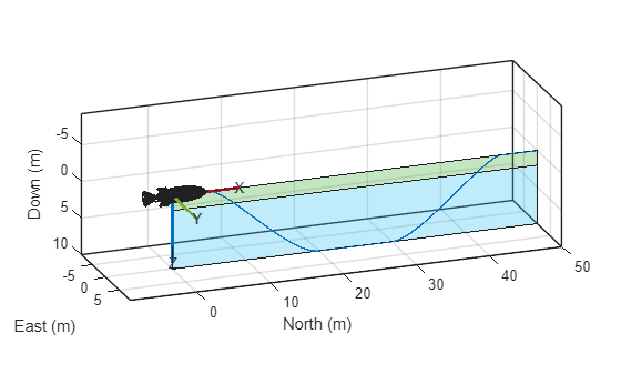
Load the predetermined ground-truth data, which serves as the reference for pose estimation. In this example, the AUV dives to a specific depth and then resurfaces. The variable groundTruth provides the ground-truth data as a timetable that contains values for the AUV position, orientation, velocity, acceleration, and angular velocity, all sampled at an IMU rate of 50 Hz. The ground-truth data also includes the variable gpsDepth, which specifies a depth of 2 meters below the water surface, where GPS sensor readings are available.

load("groundTruthForAUVPoseEstimation.mat")

Visualize the 3-D trajectory of the vehicle using the visualizeTrajectory helper function. The resulting plot highlights portions of the trajectory where GPS is available in the green shaded area.

hpose = visualizeTrajectory(groundTruth,gpsDepth)

Figure contains an axes object. The axes object with xlabel North (m), ylabel East (m) contains 3 objects of type line, patch.

hpose = 
  PosePatch with properties:

     Orientation: [1×1 quaternion]
        Position: [0 0 0]
    MeshFileName: "auv.stl"

  Use GET to show all properties

Create Extended Kalman Filter for Sensor Fusion

Create an insEKF object to represent an extended Kalman filter for sensor fusion. Use the following built-in objects to model sensor measurements:

insAccelerometer (Navigation Toolbox) — Accelerometer readings, including gravitational acceleration and sensor bias.
insGyroscope (Navigation Toolbox) — Gyroscope readings, including the angular velocity vector and sensor bias.
insMagnetometer (Navigation Toolbox) — Magnetometer readings, including the geomagnetic vector and sensor bias.
insGPS (Navigation Toolbox) — GPS readings, including latitude, longitude, and altitude coordinates. This insGPS object enables the insEKF object to fuse position and velocity data.
insMotionPose (Navigation Toolbox) — 3-D motion, assuming constant angular velocity and constant linear acceleration.

In addition to the built-in sensor models, define the following custom sensor models (attached as .m files in this example):

insDepth — Depth measurements along the z-axis of the AUV body
insSpeed — Flow-relative speed measurements along the x-axis of the AUV body
insZuptVyz — Zero-velocity updates for the y- and z-axes of the AUV body

filt = insEKF(insAccelerometer,insGyroscope,insMagnetometer, ...
    insGPS,insDepth,insSpeed,insZuptVyz,insMotionPose);

Load Sensor Data

Load prerecorded sensor data for the simulation. The variable sensorData provides the sensor data as a timetable that contains noisy readings from the accelerometer, gyroscope, magnetometer, and GPS (including velocity data in the navigation frame), as well as depth along the z-axis, flow-relative speed along the x-axis, and zero-velocity updates for the y- and z-axes of the AUV body. For the accelerometer, gyroscope, and magnetometer, the sensor data is sampled at the IMU rate of 50 Hz. The GPS readings and ZUPT data are sampled at 1 Hz. Depth and flow-relative speed data are sampled at 5 Hz.

load("sensorDataForAUVPoseEstimation.mat")

Estimate Pose of Autonomous Underwater Vehicle

Tune the process noise and measurement noise parameters of the insEKF object for AUV pose estimation by using the tuneAUVPoseFilter helper function with the provided sensor data and ground-truth states. This step may take several minutes, depending on the data size and filter complexity.

tic
[tunedFilter,tunedMeasNoise] = tuneAUVPoseFilter(filt,sensorData, ...
groundTruth(:,["Position" "Orientation"]));

Code generation successful.

    Iteration    Parameter                    Metric
    _________    _________                    ______
    1            AdditiveProcessNoise(1)      2.3712
    1            AdditiveProcessNoise(33)     2.3712
    1            AdditiveProcessNoise(65)     2.3711
    1            AdditiveProcessNoise(97)     2.3711
    1            AdditiveProcessNoise(129)    2.3711
    1            AdditiveProcessNoise(161)    2.3711
    1            AdditiveProcessNoise(193)    2.3711
    1            AdditiveProcessNoise(225)    2.3699
    1            AdditiveProcessNoise(257)    2.3698
    1            AdditiveProcessNoise(289)    2.3685
    1            AdditiveProcessNoise(321)    2.3673
    1            AdditiveProcessNoise(353)    2.3673
    1            AdditiveProcessNoise(385)    2.3665
    1            AdditiveProcessNoise(417)    2.3665
    1            AdditiveProcessNoise(449)    2.3665
    1            AdditiveProcessNoise(481)    2.3664
    1            AdditiveProcessNoise(513)    2.3664
    1            AdditiveProcessNoise(545)    2.3664
    1            AdditiveProcessNoise(577)    2.3664
    1            AdditiveProcessNoise(609)    2.3664
    1            AdditiveProcessNoise(641)    2.3664
    1            AdditiveProcessNoise(673)    2.3664
    1            AdditiveProcessNoise(705)    2.3664
    1            AdditiveProcessNoise(737)    2.3664
    1            AdditiveProcessNoise(769)    2.3664
    1            AdditiveProcessNoise(801)    2.3664
    1            AdditiveProcessNoise(833)    2.3664
    1            AdditiveProcessNoise(865)    2.3664
    1            AdditiveProcessNoise(897)    2.3319
    1            AdditiveProcessNoise(929)    2.3319
    1            AdditiveProcessNoise(961)    2.3308
    1            AccelerometerNoise           2.3307
    1            GyroscopeNoise               2.3307
    1            MagnetometerNoise            2.3307
    1            GPSNoise(1)                  2.3281
    1            GPSNoise(2)                  2.3281
    1            GPSNoise(3)                  2.3281
    1            GPSNoise(4)                  2.2881
    1            GPSNoise(5)                  2.2881
    1            GPSNoise(6)                  2.2875
    1            insDepthNoise                2.2875
    1            insSpeedNoise                2.2874
    1            insZuptVyzNoise              2.2874

toc

Elapsed time is 374.681080 seconds.

Estimate the state of the underwater vehicle using the tuned filter and sensor data. Also perform smoothing to refine the estimates.

tic
[stateEst,smoothEst] = estimateStates(tunedFilter,sensorData,tunedMeasNoise);
toc

Elapsed time is 13.250381 seconds.

Visualize Pose Estimations and Analyze Position Errors

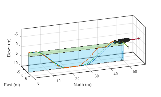
Plot the estimated position trajectories and the smoother position estimates that the tuned EKF filter produced. The smoother estimates refine the trajectory by using future measurements, which typically achieve higher accuracy.

clr = colororder;
plot3(stateEst.Position(:,1),stateEst.Position(:,2),stateEst.Position(:,3), ...
Color=clr(2,:),LineWidth=1)
plot3(smoothEst.Position(:,1),smoothEst.Position(:,2),smoothEst.Position(:,3), ...
Color=clr(5,:),LineWidth=1)

Visually compare the results. Animate the estimated trajectory and overlay it on the ground-truth trajectory by using the animateTrajectory helper function.

idx = 1:50:size(stateEst,1);
animateTrajectory(hpose,stateEst(idx,:))

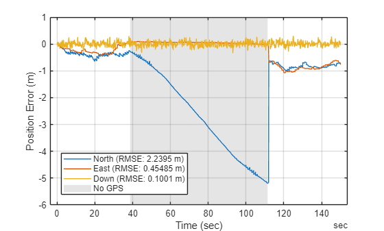
Figure contains an axes object. The axes object with xlabel North (m), ylabel East (m) contains 5 objects of type line, patch.

Compute the position errors by subtracting the ground-truth positions from the estimated positions at each time step. For each axis (North, East, Down), calculate the root mean squared error (RMSE), which summarizes the overall estimation accuracy.

posErr = stateEst.Position - groundTruth.Position;
posRmse = sqrt(mean(posErr.^2,1));

Plot the position errors of the estimated trajectories over time, displaying separate lines for each axis. Shade the regions where GPS is unavailable to highlight periods when the filter relies solely on inertial and other sensor data.

figure
plot(groundTruth.Time,posErr,LineWidth=1)
grid on
hold on

noGps = (groundTruth.Position(:,3) > gpsDepth);
tNoGps = groundTruth.Time(noGps);
xregion(tNoGps(1),tNoGps(end),FaceAlpha=0.2)

Specify the legend text and add the legend to the plot. Label the x-axis and y-axis of the plot.

legendTxt = ["North" "East" "Down"] + " (RMSE: " + posRmse + " m)";
legendTxt = [legendTxt "No GPS"];
legend(legendTxt,Location="best")
xlabel("Time (sec)")
ylabel("Position Error (m)")

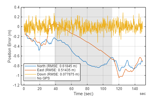
Figure contains an axes object. The axes object with xlabel Time (sec), ylabel Position Error (m) contains 4 objects of type line, constantregion. These objects represent North (RMSE: 2.2395 m), East (RMSE: 0.45485 m), Down (RMSE: 0.1001 m), No GPS.

Repeat the error computation for the smoother position estimates. Plot the smoother position errors. The smoother position estimates result in lower RMSE because these estimates use information from the entire trajectory, not just past measurements.

posErr = smoothEst.Position - groundTruth.Position;
posRmse = sqrt(mean(posErr.^2,1));
figure
plot(groundTruth.Time,posErr,LineWidth=1)
grid on
hold on
noGps = (groundTruth.Position(:,3) > gpsDepth);
tNoGps = groundTruth.Time(noGps);
xregion(tNoGps(1),tNoGps(end),FaceAlpha=0.2)
legendTxt = ["North" "East" "Down"] + " (RMSE: " + posRmse + " m)";
legendTxt = [legendTxt "No GPS"];
legend(legendTxt,Location="best")
xlabel("Time (sec)")
ylabel("Position Error (m)")

Figure contains an axes object. The axes object with xlabel Time (sec), ylabel Position Error (m) contains 4 objects of type line, constantregion. These objects represent North (RMSE: 0.61845 m), East (RMSE: 0.51435 m), Down (RMSE: 0.077875 m), No GPS.

References

[1] "Extended Kalman filter." Wikipedia, October 1, 2025. https://en.wikipedia.org/wiki/Extended_Kalman_filter.

[2] "Kalman filter." Wikipedia, October 4, 2025. https://en.wikipedia.org/wiki/Kalman_filter.

[3] "Quaternions and spatial rotation." Wikipedia, September 25, 2025. https://en.wikipedia.org/wiki/Quaternions_and_spatial_rotation.