robustfit

Fit robust linear regression

Syntax

b = robustfit(X,y)

b = robustfit(X,y,wfun,tune,const)

[b,stats] = robustfit(___)

Description

b = robustfit(X,y) returns a vector b of coefficient estimates for a robust multiple linear regression of the responses in vector y on the predictors in matrix X.

b = robustfit(X,y,wfun,tune,const) specifies the fitting weight function options wfun and tune, and the indicator const, which determines if the model includes a constant term. You can pass in [] for wfun, tune, and const to use their default values.

[b,stats] = robustfit(___) also returns a structure stats containing estimated statistics, using any of the input argument combinations in previous syntaxes.

Examples

Estimate Robust Regression Coefficients

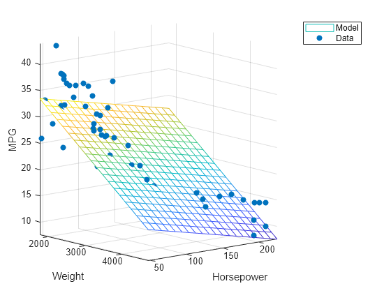
Estimate robust regression coefficients for a multiple linear model.

Load the carsmall data set. Specify car weight and horsepower as predictors and mileage per gallon as the response.

load carsmall
x1 = Weight;
x2 = Horsepower;
X = [x1 x2];
y = MPG;

Compute the robust regression coefficients.

b = robustfit(X,y)

b = 3×1

   47.1975
   -0.0068
   -0.0333

Plot the fitted model.

x1fit = linspace(min(x1),max(x1),20);
x2fit = linspace(min(x2),max(x2),20);
[X1FIT,X2FIT] = meshgrid(x1fit,x2fit);
YFIT = b(1) + b(2)*X1FIT + b(3)*X2FIT;
mesh(X1FIT,X2FIT,YFIT)

Plot the data.

hold on
scatter3(x1,x2,y,'filled')
hold off
xlabel('Weight')
ylabel('Horsepower')
zlabel('MPG')
legend('Model','Data')
view(50,10)
axis tight

Tune Robust Weight Function

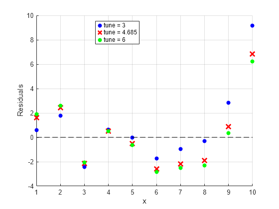
Tune the weight function for robust regression by using different tuning constants.

Generate data with the trend $$y=10-2x$$, and then change one value to simulate an outlier.

x = (1:10)';
rng ('default') % For reproducibility
y = 10 - 2*x + randn(10,1);
y(10) = 0;

Compute the robust regression residuals using the bisquare weight function for three different tuning constants. The default tuning constant is 4.685.

tune_const = [3 4.685 6];

for i = 1:length(tune_const)
    [~,stats] = robustfit(x,y,'bisquare',tune_const(i));
    resids(:,i) = stats.resid;
end

Create a plot of the residuals.

scatter(x,resids(:,1),'b','filled')
hold on
plot(resids(:,2),'rx','MarkerSize',10,'LineWidth',2)
scatter(x,resids(:,3),'g','filled')
plot([min(x) max(x)],[0 0],'--k')
hold off 
grid on
xlabel('x')
ylabel('Residuals')
legend('tune = 3','tune = 4.685','tune = 6','Location','best')

Compute the root mean squared error (RMSE) of residuals for the three different tuning constants.

rmse = sqrt(mean(resids.^2))

rmse = 1×3

    3.2577    2.7576    2.7099

Because increasing the tuning constant decreases the downweight assigned to outliers, the RMSE decreases as the tuning constant increases.

Compare Robust and Least-Squares Regression

Generate data with the trend $$y=10-2x$$, and then change one value to simulate an outlier.

x = (1:10)';
rng('default') % For reproducibility
y = 10 - 2*x + randn(10,1);
y(10) = 0;

Fit a straight line using ordinary least-squares regression. To compute coefficient estimates for a model with a constant term, include a column of ones in x.

bls = regress(y,[ones(10,1) x])

bls = 2×1

    7.8518
   -1.3644

Estimate a straight-line fit using robust regression. robustfit adds a constant term to the model by default.

[brob,stats] = robustfit(x,y);
brob

brob = 2×1

    8.4504
   -1.5278

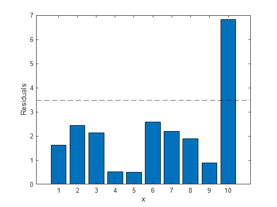
Identify potential outliers by comparing the residuals to the median absolute deviation of the residuals.

outliers_ind = find(abs(stats.resid)>stats.mad_s);

Plot a bar graph of the residuals for robust regression.

bar(abs(stats.resid))
hold on
yline(stats.mad_s,'k--')
hold off
xlabel('x')
ylabel('Residuals')

Create a scatter plot of the data.

scatter(x,y,'filled')

Plot the outlier.

hold on 
plot(x(outliers_ind),y(outliers_ind),'mo','LineWidth',2)

Plot the least-squares and robust fit.

plot(x,bls(1)+bls(2)*x,'r')
plot(x,brob(1)+brob(2)*x,'g')
hold off
xlabel('x')
ylabel('y')
legend('Data','Outlier','Ordinary Least Squares','Robust Regression')
grid on

The outlier influences the robust fit less than the least-squares fit.

Input Arguments

X — Predictor data

numeric matrix

Predictor data, specified as an n-by-p numeric matrix. Rows of X correspond to observations, and columns correspond to predictor variables. X must have the same number of rows as y.

By default, robustfit adds a constant term to the model, unless you explicitly remove it by specifying const as 'off'. So, do not include a column of 1s in X.

Data Types: single | double

y — Response data

numeric vector

Response data, specified as an n-by-1 numeric vector. Rows of y correspond to different observations. y must have the same number of rows as X.

Data Types: single | double

wfun — Robust fitting weight function

'bisquare' (default) | 'andrews' | 'cauchy' | 'fair' | function handle | ...

Robust fitting weight function, specified as the name of a weight function described in the following table, or a function handle. robustfit uses the corresponding default tuning constant, unless otherwise specified by tune.

Weight Function	Description	Default Tuning Constant
'andrews'	w = (abs(r)<pi) .* sin(r) ./ r	1.339
'bisquare'	w = (abs(r)<1) .* (1 - r.^2).^2 (also called biweight)	4.685
'cauchy'	w = 1 ./ (1 + r.^2)	2.385
'fair'	w = 1 ./ (1 + abs(r))	1.400
'huber'	w = 1 ./ max(1, abs(r))	1.345
'logistic'	w = tanh(r) ./ r	1.205
'ols'	Ordinary least squares (no weighting function)	None
'talwar'	w = 1 * (abs(r)<1)	2.795
'welsch'	w = exp(-(r.^2))	2.985
function handle	Custom weight function that accepts a vector r of scaled residuals, and returns a vector of weights the same size as r	1

The value r in the weight functions is

r = resid/(tune*s*sqrt(1–h)),

where

• resid is the vector of residuals from the previous iteration.

• tune is the tuning constant.

• h is the vector of leverage values from a least-squares fit.

• s is an estimate of the standard deviation of the error term given by s = MAD/0.6745.

MAD is the median absolute deviation of the residuals from their median. The constant 0.6745 makes the estimate unbiased for the normal distribution. If X has p columns, the software excludes the smallest p absolute deviations when computing the median.

Data Types: char | string | function handle

tune — Tuning constant

positive scalar

Tuning constant, specified as a positive scalar. If you do not set tune, robustfit uses the corresponding default tuning constant for each weight function (see the table in wfun).

The default tuning constants of built-in weight functions give coefficient estimates that are approximately 95% as statistically efficient as the ordinary least-squares estimates, provided that the response has a normal distribution with no outliers. Decreasing the tuning constant increases the downweight assigned to large residuals; increasing the tuning constant decreases the downweight assigned to large residuals.

Data Types: single | double

const — Indicator for constant term

'on' (default) | 'off'

Indicator for a constant term in the fit, specified as 'on' or 'off'. If const is 'on', then robustfit adds a first column of 1s to the predictor matrix X, and the output b becomes a (p + 1)-by-1 vector. If const is 'off', then X remains unchanged and b is a p-by-1 vector.

Data Types: char | string

Output Arguments

b — Coefficient estimates for robust multiple linear regression

numeric vector

Coefficient estimates for robust multiple linear regression, returned as a numeric vector. b is a p-by-1 vector, where p is the number of predictors in X.

By default, robustfit adds a constant term to the model, unless you explicitly remove it by specifying const as 'off'.

stats — Model statistics

structure

Model statistics, returned as a structure. The following table describes the fields of the diagnostic statistics structure from the robust regression.

Field	Description
ols_s	Sigma estimate (root mean squared error) from ordinary least squares
robust_s	Robust estimate of sigma
mad_s	Estimate of sigma computed using the median absolute deviation of the residuals from their median; used for scaling residuals during iterative fitting
s	Final estimate of sigma, the largest between robust_s and a weighted average of ols_s and robust_s
resid	Residuals, observed minus fitted values (see Raw Residuals)
rstud	Studentized residuals, the residuals divided by an independent estimate of the residual standard deviation (see Studentized Residuals)
se	Standard error of the estimated coefficient value b
covb	Estimated covariance matrix for coefficient estimates
coeffcorr	Estimated correlation of coefficient estimates
t	t-statistic for each coefficient to test the null hypothesis that the corresponding coefficient is zero against the alternative that it is different from zero, given the other predictors in the model. Note that t = b/se.
p	p-values for the t-statistic of the hypothesis test that the corresponding coefficient is equal to zero or not
w	Vector of weights for a robust fit
R	R factor in the QR decomposition of X
dfe	Degrees of freedom for the error (residuals), equal to the number of observations minus the number of estimated coefficients
h	Vector of leverage values for a least-squares fit

More About

Leverage

Leverage is a measure of the effect of a particular observation on the regression predictions due to the position of that observation in the space of the inputs.

The leverage of observation i is the value of the ith diagonal term h_ii of the hat matrix H. The hat matrix H is defined in terms of the data matrix X:

H = X(X^TX)^–1X^T.

The hat matrix is also known as the projection matrix because it projects the vector of observations y onto the vector of predictions $$\widehat{y}$$, thus putting the "hat" on y.

Because the sum of the leverage values is p (the number of coefficients in the regression model), an observation i can be considered an outlier if its leverage substantially exceeds p/n, where n is the number of observations.

For more details, see Hat Matrix and Leverage.

Tips

• robustfit treats NaN values in X or y as missing values. robustfit omits observations with missing values from the robust fit.

Algorithms

• robustfit uses iteratively reweighted least squares to compute the coefficients b. The input wfun specifies the weights.

• robustfit estimates the variance-covariance matrix of the coefficient estimates stats.covb using the formula inv(X'*X)*stats.s^2. This estimate produces the standard error stats.se and correlation stats.coeffcorr.

• In a linear model, observed values of y and their residuals are random variables. Residuals have normal distributions with zero mean but with different variances at different values of the predictors. To put residuals on a comparable scale, robustfit “Studentizes” the residuals. That is, robustfit divides the residuals by an estimate of their standard deviation that is independent of their value. Studentized residuals have t-distributions with known degrees of freedom. robustfit returns the Studentized residuals in stats.rstud.

Alternative Functionality

robustfit is useful when you simply need the output arguments of the function or when you want to repeat fitting a model multiple times in a loop. If you need to investigate a robust fitted regression model further, create a linear regression model object LinearModel by using fitlm. Set the value for the name-value pair argument 'RobustOpts' to 'on'.

References

[1] DuMouchel, W. H., and F. L. O'Brien. “Integrating a Robust Option into a Multiple Regression Computing Environment.” Computer Science and Statistics: Proceedings of the 21st Symposium on the Interface. Alexandria, VA: American Statistical Association, 1989.

[2] Holland, P. W., and R. E. Welsch. “Robust Regression Using Iteratively Reweighted Least-Squares.” Communications in Statistics: Theory and Methods, A6, 1977, pp. 813–827.

[3] Huber, P. J. Robust Statistics. Hoboken, NJ: John Wiley & Sons, Inc., 1981.

[4] Street, J. O., R. J. Carroll, and D. Ruppert. “A Note on Computing Robust Regression Estimates via Iteratively Reweighted Least Squares.” The American Statistician. Vol. 42, 1988, pp. 152–154.

Version History

Introduced before R2006a