Perform Nonnegative Matrix Factorization
This example shows how to perform nonnegative matrix factorization.
Load the sample data.
load moore
X = moore(:,1:5);
rng('default'); % For reproducibility
Compute a rank-two approximation of X using a multiplicative update algorithm that begins from five random initial values for W and H.
opt = statset('MaxIter',10,'Display','final');
[W0,H0] = nnmf(X,2,'replicates',5,'options',opt,'algorithm','mult');
    rep	   iteration	   rms resid	  |delta x|
      1	      10	     358.296	  0.00190554
      2	      10	     78.3556	 0.000351747
      3	      10	     230.962	   0.0172839
      4	      10	     326.347	  0.00739552
      5	      10	     361.547	  0.00705539
Final root mean square residual = 78.3556
The 'mult' algorithm is sensitive to initial values, which makes it a good choice when using 'replicates' to find W and H from multiple random starting values.
Now perform the factorization using alternating least-squares algorithm, which converges faster and more consistently. Run 100 times more iterations, beginning from the initial W0 and H0 identified above.
opt = statset('Maxiter',1000,'Display','final');
[W,H] = nnmf(X,2,'w0',W0,'h0',H0,'options',opt,'algorithm','als');
    rep	   iteration	   rms resid	  |delta x|
      1	       2	     77.5315	 0.000830334
Final root mean square residual = 77.5315
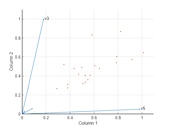
The two columns of W are the transformed predictors. The two rows of H give the relative contributions of each of the five predictors in X to the predictors in W. Display H.
H
H = 2×5

    0.0835    0.0190    0.1782    0.0072    0.9802
    0.0559    0.0250    0.9969    0.0085    0.0497
The fifth predictor in X (weight 0.9802) strongly influences the first predictor in W. The third predictor in X (weight 0.9969) strongly influences the second predictor in W.
Visualize the relative contributions of the predictors in X with biplot, showing the data and original variables in the column space of W.
biplot(H','scores',W,'varlabels',{'','','v3','','v5'});
axis([0 1.1 0 1.1])
xlabel('Column 1')
ylabel('Column 2')
