incrementalClassificationNaiveBayes
Naive Bayes classification model for incremental learning
Description
The incrementalClassificationNaiveBayes function creates an
incrementalClassificationNaiveBayes model object, which represents a naive Bayes multiclass
classification model for incremental learning.
Unlike other Statistics and Machine Learning Toolbox™ model objects, incrementalClassificationNaiveBayes can be called directly. Also,
you can specify learning options, such as performance metrics configurations and prior class
probabilities, before fitting the model to data. After you create an
incrementalClassificationNaiveBayes object, it is prepared for incremental learning.
incrementalClassificationNaiveBayes is best suited for incremental learning. For a traditional
approach to training a naive Bayes model for multiclass classification (such as creating a
model by fitting it to data, performing cross-validation, tuning hyperparameters, and so on),
see fitcnb.
Creation
You can create an incrementalClassificationNaiveBayes model object in several ways:
Call the function directly — Configure incremental learning options, or specify learner-specific options, by calling
incrementalClassificationNaiveBayesdirectly. This approach is best when you do not have data yet or you want to start incremental learning immediately. You must specify the maximum number of classes or all class names expected in the response data during incremental learning.Convert a traditionally trained model — To initialize a naive Bayes classification model for incremental learning using the model parameters of a trained model object (
ClassificationNaiveBayes), you can convert the traditionally trained model to anincrementalClassificationNaiveBayesmodel object by passing it to theincrementalLearnerfunction.Call an incremental learning function —
fit,updateMetrics, andupdateMetricsAndFitaccept a configuredincrementalClassificationNaiveBayesmodel object and data as input, and return anincrementalClassificationNaiveBayesmodel object updated with information learned from the input model and data.
Syntax
Description
Mdl = incrementalClassificationNaiveBayes('MaxNumClasses',MaxNumClasses)Mdl, where MaxNumClasses is the maximum number
of classes expected in the response data during incremental learning. Properties of a
default model contain placeholders for unknown model parameters. You must train a default
model before you can track its performance or generate predictions from it.
Mdl = incrementalClassificationNaiveBayes('ClassNames',ClassNames)ClassNames expected in the response data during incremental learning, and sets the ClassNames property.
Mdl = incrementalClassificationNaiveBayes(___,Name,Value)incrementalClassificationNaiveBayes('DistributionNames','mn','MaxNumClasses',5,'MetricsWarmupPeriod',100)
specifies that the joint conditional distribution of the predictor variables is
multinomial, sets the maximum number of classes expected in the response data to
5, and sets the metrics warm-up period to
100.
Input Arguments
Name-Value Arguments
Properties
Object Functions
fit | Train naive Bayes classification model for incremental learning |
updateMetricsAndFit | Update performance metrics in naive Bayes incremental learning classification model given new data and train model |
updateMetrics | Update performance metrics in naive Bayes incremental learning classification model given new data |
logp | Log unconditional probability density of naive Bayes classification model for incremental learning |
loss | Loss of naive Bayes incremental learning classification model on batch of data |
predict | Predict responses for new observations from naive Bayes incremental learning classification model |
perObservationLoss | Per observation classification error of model for incremental learning |
reset | Reset incremental classification model |
Examples
To create a naive Bayes classification model for incremental learning, you must specify the maximum number of classes that you expect the model to process ('MaxNumClasses' name-value argument). As you fit the model to incoming batches of data by using an incremental fitting function, the model collects new classes in its ClassNames property. If the specified maximum number of classes is inaccurate, one of the following occurs:
Before an incremental fitting function processes the expected maximum number of classes, the model is cold. Consequently, the
updateMetricsandupdateMetricsAndFitfunctions do not measure performance metrics.If the number of classes exceeds the maximum expected, the incremental fitting function issues an error.
This example shows how to create a naive Bayes classification model for incremental learning when the only information you specify is the expected maximum number of classes in the data. Also, the example illustrates the consequences when incremental fitting functions process all expected classes early and late in the sample.
For this example, consider training a device to predict whether a subject is sitting, standing, walking, running, or dancing based on biometric data measured on the subject. Therefore, the device has a maximum of 5 classes from which to choose.
Process Expected Maximum Number of Classes Early in Sample
Create an incremental naive Bayes model for multiclass learning. Specify a maximum of 5 classes in the data.
MdlEarly = incrementalClassificationNaiveBayes('MaxNumClasses',5)MdlEarly =
incrementalClassificationNaiveBayes
IsWarm: 0
Metrics: [1×2 table]
ClassNames: [1×0 double]
ScoreTransform: 'none'
DistributionNames: 'normal'
DistributionParameters: {}
Properties, Methods
MdlEarly is an incrementalClassificationNaiveBayes model object. All its properties are read-only.
MdlEarly must be fit to data before you can use it to perform any other operations.
Load the human activity data set. Randomly shuffle the data.
load humanactivity
n = numel(actid);
rng(1); % For reproducibility
idx = randsample(n,n);
X = feat(idx,:);
Y = actid(idx);
For details on the data set, enter Description at the command line.
Fit the incremental model to the training data by using the updateMetricsAndFit function. Simulate a data stream by processing chunks of 50 observations at a time. At each iteration:
Process 50 observations.
Overwrite the previous incremental model with a new one fitted to the incoming observations.
Store the mean of the first predictor in the first class , the cumulative metrics, and the window metrics to see how they evolve during incremental learning.
% Preallocation
numObsPerChunk = 50;
nchunk = floor(n/numObsPerChunk);
mc = array2table(zeros(nchunk,2),'VariableNames',["Cumulative" "Window"]);
mu1 = zeros(nchunk+1,1);

% Incremental learning
for j = 1:nchunk
    ibegin = min(n,numObsPerChunk*(j-1) + 1);
    iend = min(n,numObsPerChunk*j);
    idx = ibegin:iend;
    MdlEarly = updateMetricsAndFit(MdlEarly,X(idx,:),Y(idx));
    mc{j,:} = MdlEarly.Metrics{"MinimalCost",:};
    mu1(j + 1) = MdlEarly.DistributionParameters{1,1}(1);
end
MdlEarly is an incrementalClassificationNaiveBayes model object trained on all the data in the stream. During incremental learning and after the model is warmed up, updateMetricsAndFit checks the performance of the model on the incoming observations, and then fits the model to those observations.
To see how the performance metrics and evolve during training, plot them on separate tiles.
t = tiledlayout(2,1);
nexttile
plot(mu1)
ylabel('\mu_{11}')
xlim([0 nchunk])
nexttile
h = plot(mc.Variables);
xlim([0 nchunk])
ylabel('Minimal Cost')
xline(MdlEarly.MetricsWarmupPeriod/numObsPerChunk,'r-.')
legend(h,mc.Properties.VariableNames)
xlabel(t,'Iteration')
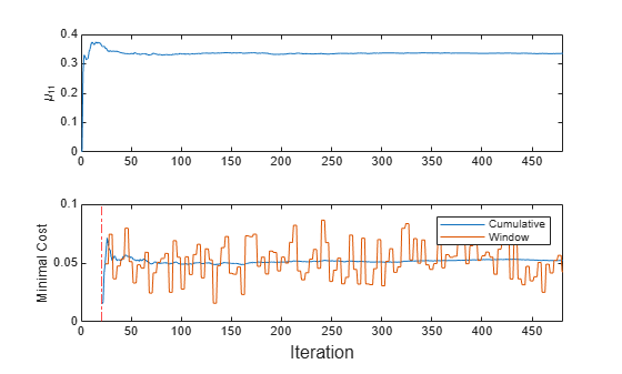
The plots indicate that updateMetricsAndFit performs the following actions:
Fit during all incremental learning iterations.
Compute the performance metrics after the metrics warm-up period (red vertical line) only.
Compute the cumulative metrics during each iteration.
Compute the window metrics after processing 200 observations (4 iterations).
Process Expected Maximum Number of Classes Late in Sample
Create a different naive Bayes model for incremental learning for the objective.
MdlLate = incrementalClassificationNaiveBayes('MaxNumClasses',5)MdlLate =
incrementalClassificationNaiveBayes
IsWarm: 0
Metrics: [1×2 table]
ClassNames: [1×0 double]
ScoreTransform: 'none'
DistributionNames: 'normal'
DistributionParameters: {}
Properties, Methods
Move all observations labeled with class 5 to the end of the sample.
idx5 = Y == 5;
Xnew = [X(~idx5,:); X(idx5,:)];
Ynew = [Y(~idx5) ;Y(idx5)];
Fit the incremental model and plot the results.
mcnew = array2table(zeros(nchunk,2),'VariableNames',["Cumulative" "Window"]);
mu1new = zeros(nchunk,1);

for j = 1:nchunk
    ibegin = min(n,numObsPerChunk*(j-1) + 1);
    iend   = min(n,numObsPerChunk*j);
    idx = ibegin:iend;
    MdlLate = updateMetricsAndFit(MdlLate,Xnew(idx,:),Ynew(idx));
    mcnew{j,:} = MdlLate.Metrics{"MinimalCost",:};
    mu1new(j + 1) = MdlLate.DistributionParameters{1,1}(1);
end

t = tiledlayout(2,1);
nexttile
plot(mu1new)
ylabel('\mu_{11}')
xlim([0 nchunk])
nexttile
h = plot(mcnew.Variables);
xlim([0 nchunk]);
ylabel('Minimal Cost')
xline(MdlLate.MetricsWarmupPeriod/numObsPerChunk,'r-.')
xline(sum(~idx5)/numObsPerChunk,'g-.')
legend(h,mcnew.Properties.VariableNames,'Location','best')
xlabel(t,'Iteration')
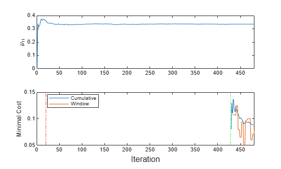
The updateMetricsAndFit function trains the model throughout incremental learning, but the function starts tracking performance metrics only after the model is fit to all expected number of classes (the green vertical line in the bottom tile).
Create an incremental naive Bayes model when you know all the class names in the data.
Consider training a device to predict whether a subject is sitting, standing, walking, running, or dancing based on biometric data measured on the subject. The class names map 1 through 5 to an activity.
Create an incremental naive Bayes model for multiclass learning. Specify the class names.
classnames = 1:5;
Mdl = incrementalClassificationNaiveBayes('ClassNames',classnames)
Mdl =
incrementalClassificationNaiveBayes
IsWarm: 0
Metrics: [1×2 table]
ClassNames: [1 2 3 4 5]
ScoreTransform: 'none'
DistributionNames: 'normal'
DistributionParameters: {5×0 cell}
Properties, Methods
Mdl is an incrementalClassificationNaiveBayes model object. All its properties are read-only.
Mdl must be fit to data before you can use it to perform any other operations.
Load the human activity data set. Randomly shuffle the data.
load humanactivity
n = numel(actid);
rng(1); % For reproducibility
idx = randsample(n,n);
X = feat(idx,:);
Y = actid(idx);
For details on the data set, enter Description at the command line.
Fit the incremental model to the training data by using the updateMetricsAndFit function. Simulate a data stream by processing chunks of 50 observations at a time. At each iteration:
Process 50 observations.
Overwrite the previous incremental model with a new one fitted to the incoming observations.
% Preallocation
numObsPerChunk = 50;
nchunk = floor(n/numObsPerChunk);

% Incremental learning
for j = 1:nchunk
    ibegin = min(n,numObsPerChunk*(j-1) + 1);
    iend   = min(n,numObsPerChunk*j);
    idx = ibegin:iend;
    Mdl = updateMetricsAndFit(Mdl,X(idx,:),Y(idx));
end
In addition to specifying the maximum number of class names, prepare an incremental naive Bayes learner by specifying a metrics warm-up period, during which the updateMetricsAndFit function fits only the model. Specify a metrics window size of 500 observations.
Load the human activity data set. Randomly shuffle the data.
load humanactivity
n = numel(actid);
rng(1); % For reproducibility
idx = randsample(n,n);
X = feat(idx,:);
Y = actid(idx);
The class names map 1 through 5 to an activity—sitting, standing, walking, running, or dancing, respectively—based on biometric data measured on the subject. For details on the data set, enter Description at the command line.
Create an incremental naive Bayes model for multiclass learning. Configure the model as follows:
Specify a metrics warm-up period of 5000 observations.
Specify a metrics window size of 500 observations.
Double the penalty to the classifier when it mistakenly classifies class 2.
Track the classification error and minimal cost to measure the performance of the model. You do not have to specify
'mincost'forMetricsbecauseincrementalClassificationNaiveBayesalways tracks this metric.
C = ones(5) - eye(5);
C(2,[1 3 4 5]) = 2;
Mdl = incrementalClassificationNaiveBayes('ClassNames',1:5, ...
    'MetricsWarmupPeriod',5000,'MetricsWindowSize',500, ...
    'Cost',C,'Metrics','classiferror')
Mdl =
  incrementalClassificationNaiveBayes

                    IsWarm: 0
                   Metrics: [2×2 table]
                ClassNames: [1 2 3 4 5]
            ScoreTransform: 'none'
         DistributionNames: 'normal'
    DistributionParameters: {5×0 cell}


  Properties, Methods
Mdl is an incrementalClassificationNaiveBayes model object configured for incremental learning.
Fit the incremental model to the rest of the data by using the updateMetricsAndFit function. At each iteration:
Simulate a data stream by processing a chunk of 50 observations.
Overwrite the previous incremental model with a new one fitted to the incoming observations.
Store the standard deviation of the first predictor variable in the first class , the cumulative metrics, and the window metrics to see how they evolve during incremental learning.
% Preallocation
numObsPerChunk = 50;
nchunk = floor(n/numObsPerChunk);
ce = array2table(zeros(nchunk,2),'VariableNames',["Cumulative" "Window"]);
mc = array2table(zeros(nchunk,2),'VariableNames',["Cumulative" "Window"]);
sigma11 = zeros(nchunk+1,1);

% Incremental fitting
for j = 1:nchunk
    ibegin = min(n,numObsPerChunk*(j-1) + 1);
    iend   = min(n,numObsPerChunk*j);
    idx = ibegin:iend;
    Mdl = updateMetricsAndFit(Mdl,X(idx,:),Y(idx));
    ce{j,:} = Mdl.Metrics{"ClassificationError",:};
    mc{j,:} = Mdl.Metrics{"MinimalCost",:};
    sigma11(j + 1) = Mdl.DistributionParameters{1,1}(2);
end
Mdl is an incrementalClassificationNaiveBayes model object trained on all the data in the stream. During incremental learning and after the model is warmed up, updateMetricsAndFit checks the performance of the model on the incoming observations, and then fits the model to those observations.
To see how the performance metrics and evolve during training, plot them on separate tiles.
tiledlayout(2,2)
nexttile
plot(sigma11)
ylabel('\sigma_{11}')
xlim([0 nchunk]);
xline(Mdl.MetricsWarmupPeriod/numObsPerChunk,'r-.')
xlabel('Iteration')
nexttile
h = plot(ce.Variables);
xlim([0 nchunk])
ylabel('Classification Error')
xline(Mdl.MetricsWarmupPeriod/numObsPerChunk,'r-.')
legend(h,ce.Properties.VariableNames)
xlabel('Iteration')
nexttile
h = plot(mc.Variables);
xlim([0 nchunk]);
ylabel('Minimal Cost')
xline(Mdl.MetricsWarmupPeriod/numObsPerChunk,'r-.')
legend(h,mc.Properties.VariableNames)
xlabel('Iteration')
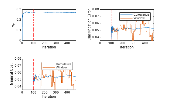
The plots indicate that updateMetricsAndFit performs the following actions:
Fit during all incremental learning iterations.
Compute the performance metrics after the metrics warm-up period (red vertical line) only.
Compute the cumulative metrics during each iteration.
Compute the window metrics after processing 500 observations (10 iterations).
Train a naive Bayes model for multiclass classification by using fitcnb. Then, convert the model to an incremental learner, track its performance, and fit the model to streaming data. Carry over training options from traditional to incremental learning.
Load and Preprocess Data
Load the human activity data set. Randomly shuffle the data.
load humanactivity
rng(1) % For reproducibility
n = numel(actid);
idx = randsample(n,n);
X = feat(idx,:);
Y = actid(idx);
For details on the data set, enter Description at the command line.
Suppose that the data collected when the subject was idle (Y <= 2) has double the quality than when the subject was moving. Create a weight variable that attributes 2 to observations collected from an idle subject, and 1 to a moving subject.
W = ones(n,1) + (Y <= 2);
Train Naive Bayes Model
Fit a naive Bayes model for multiclass classification to a random sample of half the data.
idxtt = randsample([true false],n,true);
TTMdl = fitcnb(X(idxtt,:),Y(idxtt),'Weights',W(idxtt))
TTMdl =
ClassificationNaiveBayes
ResponseName: 'Y'
CategoricalPredictors: []
ClassNames: [1 2 3 4 5]
ScoreTransform: 'none'
NumObservations: 12053
DistributionNames: {1×60 cell}
DistributionParameters: {5×60 cell}
Properties, Methods
TTMdl is a ClassificationNaiveBayes model object representing a traditionally trained naive Bayes model.
Convert Trained Model
Convert the traditionally trained naive Bayes model to a naive Bayes classification model for incremental learning.
IncrementalMdl = incrementalLearner(TTMdl)
IncrementalMdl =
  incrementalClassificationNaiveBayes

                    IsWarm: 1
                   Metrics: [1×2 table]
                ClassNames: [1 2 3 4 5]
            ScoreTransform: 'none'
         DistributionNames: {1×60 cell}
    DistributionParameters: {5×60 cell}


  Properties, Methods
Separately Track Performance Metrics and Fit Model
Perform incremental learning on the rest of the data by using the updateMetrics and fit functions. Simulate a data stream by processing 50 observations at a time. At each iteration:
Call
updateMetricsto update the cumulative and window classification error of the model given the incoming chunk of observations. Overwrite the previous incremental model to update the losses in theMetricsproperty. Note that the function does not fit the model to the chunk of data—the chunk is "new" data for the model. Specify the observation weights.Call
fitto fit the model to the incoming chunk of observations. Overwrite the previous incremental model to update the model parameters. Specify the observation weights.Store the minimal cost and mean of the first predictor variable of the first class .
% Preallocation
idxil = ~idxtt;
nil = sum(idxil);
numObsPerChunk = 50;
nchunk = floor(nil/numObsPerChunk);
mc = array2table(zeros(nchunk,2),'VariableNames',["Cumulative" "Window"]);
mu11 = [IncrementalMdl.DistributionParameters{1,1}(1); zeros(nchunk+1,1)];
Xil = X(idxil,:);
Yil = Y(idxil);
Wil = W(idxil);

% Incremental fitting
for j = 1:nchunk
    ibegin = min(nil,numObsPerChunk*(j-1) + 1);
    iend   = min(nil,numObsPerChunk*j);
    idx = ibegin:iend;
    IncrementalMdl = updateMetrics(IncrementalMdl,Xil(idx,:),Yil(idx), ...
        'Weights',Wil(idx));
    mc{j,:} = IncrementalMdl.Metrics{"MinimalCost",:};
    IncrementalMdl = fit(IncrementalMdl,Xil(idx,:),Yil(idx),'Weights',Wil(idx));
    mu11(j+1) = IncrementalMdl.DistributionParameters{1,1}(1);
end
IncrementalMdl is an incrementalClassificationNaiveBayes model object trained on all the data in the stream.
Alternatively, you can use updateMetricsAndFit to update the performance metrics of the model given a new chunk of data, and then fit the model to the data.
Plot a trace plot of the performance metrics and .
t = tiledlayout(2,1);
nexttile
h = plot(mc.Variables);
xlim([0 nchunk])
ylabel('Minimal Cost')
legend(h,mc.Properties.VariableNames)
nexttile
plot(mu11)
ylabel('\mu_{11}')
xlim([0 nchunk])
xlabel(t,'Iteration')
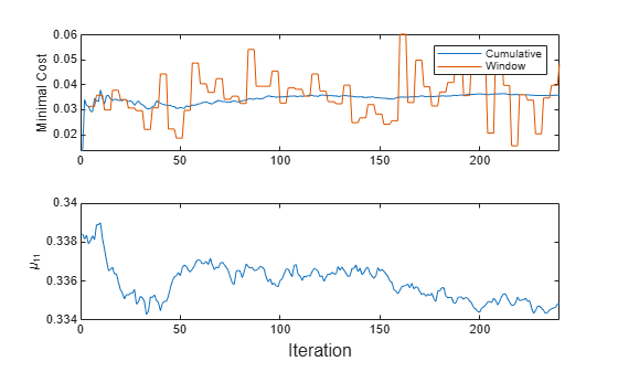
The cumulative loss levels quickly and is stable, whereas the window loss jumps throughout the training.
changes abruptly at first, then gradually levels off as fit processes more chunks.
More About
Algorithms
References
Version History
Introduced in R2021aSee Also
Functions
Topics
- Incremental Learning Overview
- Configure Incremental Learning Model
- Implement Incremental Learning for Classification Using Succinct Workflow
- Implement Incremental Learning for Classification Using Flexible Workflow
- Perform Text Classification Incrementally
- Incremental Learning with Naive Bayes and Heterogeneous Data