Generating Data Using Flexible Families of Distributions

This example shows how to generate data using the Pearson and Johnson systems of distributions.

Pearson and Johnson Systems

As described in Working with Probability Distributions, choosing an appropriate parametric family of distributions to model your data can be based on a priori or a posteriori knowledge of the data-producing process, but the choice is often difficult. The Pearson and Johnson systems can make such a choice unnecessary. Each system is a flexible parametric family of distributions that includes a wide range of distribution shapes, and it is often possible to find a distribution within one of these two systems that provides a good match to your data.

Data Input

The following parameters define each member of the Pearson and Johnson systems.

• Mean — Estimated by mean

• Standard deviation — Estimated by std

• Skewness — Estimated by skewness

• Kurtosis — Estimated by kurtosis

These statistics can also be computed with the moment function. The Johnson system, while based on these four parameters, is more naturally described using quantiles, estimated by the quantile function.

The pearsrnd and johnsrnd functions take input arguments defining a distribution (parameters or quantiles, respectively) and return the type and the coefficients of the distribution in the corresponding system. Both functions also generate random numbers from the specified distribution.

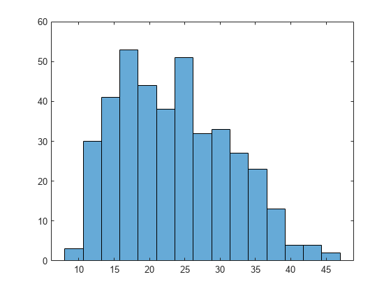
As an example, load the data in carbig.mat, which includes a variable MPG containing measurements of the gas mileage for each car.

load carbig
MPG = MPG(~isnan(MPG));
histogram(MPG,15)

The following two sections model the distribution with members of the Pearson and Johnson systems, respectively.

Generating Data Using the Pearson System

The statistician Karl Pearson devised a system, or family, of distributions that includes a unique distribution corresponding to every valid combination of mean, standard deviation, skewness, and kurtosis. If you compute sample values for each of these moments from data, it is easy to find the distribution in the Pearson system that matches these four moments and to generate a random sample.

The Pearson system embeds seven basic types of distribution together in a single parametric framework. It includes common distributions such as the normal and $$t$$ distributions, simple transformations of standard distributions such as a shifted and scaled beta distribution and the inverse gamma distribution, and one distribution—the Type IV—that is not a simple transformation of any standard distribution.

For a given set of moments, there are distributions that are not in the system that also have those same first four moments, and the distribution in the Pearson system may not be a good match to your data, particularly if the data are multimodal. But the system does cover a wide range of distribution shapes, including both symmetric and skewed distributions.

To generate a sample from the Pearson distribution that closely matches the MPG data, simply compute the four sample moments and treat those as distribution parameters.

moments = {mean(MPG),std(MPG),skewness(MPG),kurtosis(MPG)};
rng('default')  % For reproducibility
[r,type] = pearsrnd(moments{:},10000,1);

The optional second output from pearsrnd indicates which type of distribution within the Pearson system matches the combination of moments.

type

type = 
1

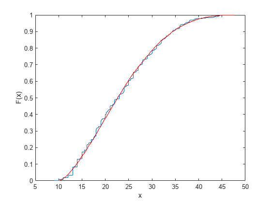
In this case, pearsrnd has determined that the data are best described with a Type I Pearson distribution, which is a shifted, scaled beta distribution.

Verify that the sample resembles the original data by overlaying the empirical cumulative distribution functions.

ecdf(MPG);
[Fi,xi] = ecdf(r);
hold on;
stairs(xi,Fi,'r');
hold off

Generating Data Using the Johnson System

Statistician Norman Johnson devised a different system of distributions that also includes a unique distribution for every valid combination of mean, standard deviation, skewness, and kurtosis. However, since it is more natural to describe distributions in the Johnson system using quantiles, working with this system is different than working with the Pearson system.

The Johnson system is based on three possible transformations of a normal random variable, plus the identity transformation. The three nontrivial cases are known as SL , SU , and SB , corresponding to exponential, logistic, and hyperbolic sine transformations. All three can be written as

$$X=\gamma +\delta \cdot \Gamma \left(\frac{Z-\xi }{\lambda }\right)$$

where $$Z$$ is a standard normal random variable, $$\Gamma$$ is the transformation, and $$\gamma$$, $$\delta$$, $$\xi$$, and $$\lambda$$ are scale and location parameters. The fourth case, SN , is the identity transformation.

To generate a sample from the Johnson distribution that matches the MPG data, first define the four quantiles to which the four evenly spaced standard normal quantiles of -1.5, -0.5, 0.5, and 1.5 should be transformed. That is, you compute the sample quantiles of the data for the cumulative probabilities of 0.067, 0.309, 0.691, and 0.933.

probs = normcdf([-1.5 -0.5 0.5 1.5])

probs = 1×4

    0.0668    0.3085    0.6915    0.9332

quantiles = quantile(MPG,probs)

quantiles = 1×4

   13.0000   18.0000   27.2000   36.0000

Then treat those quantiles as distribution parameters.

[r1,type] = johnsrnd(quantiles,10000,1);

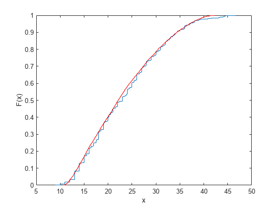
The optional second output from johnsrnd indicates which type of distribution within the Johnson system matches the quantiles.

type

type = 
'SB'

You can verify that the sample resembles the original data by overlaying the empirical cumulative distribution functions.

ecdf(MPG);
[Fi,xi] = ecdf(r1);
hold on;
stairs(xi,Fi,'r');
hold off

In some applications, it may be important to match the quantiles better in some regions of the data than in others. To do that, specify four evenly spaced standard normal quantiles at which you want to match the data, instead of the default -1.5, -0.5, 0.5, and 1.5. For example, you might care more about matching the data in the right tail than in the left, and so you specify standard normal quantiles that emphasizes the right tail.

qnorm = [-.5 .25 1 1.75];
probs = normcdf(qnorm);
qemp = quantile(MPG,probs);
r2 = johnsrnd([qnorm; qemp],10000,1);

However, while the new sample matches the original data better in the right tail, it matches much worse in the left tail.

[Fj,xj] = ecdf(r2);
hold on;
stairs(xj,Fj,'g');
hold off