fsurfht

Interactive contour plot

Syntax

fsurfht(fun,xlims,ylims)
fsurfht(fun,xlims,ylims,p1,p2,p3,p4,p5)


Description

fsurfht(fun,xlims,ylims) is an interactive contour plot of the function specified by the text variable fun. The x-axis limits are specified by xlims in the form [xmin xmax], and the y-axis limits are specified by ylims in the form [ymin ymax].

fsurfht(fun,xlims,ylims,p1,p2,p3,p4,p5) allows for five optional parameters that you can supply to the function fun.

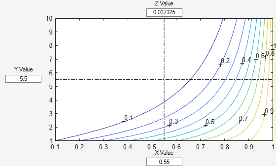
The intersection of the vertical and horizontal reference lines on the plot defines the current x value and y value. You can drag these reference lines and watch the calculated z-values (at the top of the plot) update simultaneously. Alternatively, you can type the x value and y value into editable text fields on the x-axis and y-axis.

Examples

Create Interactive Contour Plot for Specified Function

Create an interactive contour plot for a Gaussian likelihood function by using the fsurfht function.

Load the gas data set, which contains gasoline prices.

load gas

Define a function named gausslike.m that calls the normpdf function, treats the data sample as fixed, and treats the parameters mu and sigma as variables.

Display the contents of the gausslike.m file.

type gausslike.m

function z = gausslike(mu,sigma,p1)
    n = length(p1);
    z = ones(size(mu));
    for i = 1:n
        z = z.*(normpdf(p1(i),mu,sigma));
    end
end

Note: If you click the button located in the upper-right section of this page and open this example in MATLAB®, then MATLAB opens the example folder. This folder includes the gausslike.m function file for this example.

Assume that the gas prices are normally distributed, and plot the likelihood surface of the sample price1.

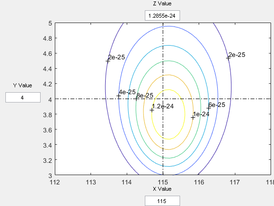
fsurfht("gausslike",[112 118],[3 5],price1)

The sample mean is the x value at the maximum, but the sample standard deviation is not the y value at the maximum. The y value at the maximum is the sample standard deviation normalized by n (instead of $n-1$), where n is the number of observations in the sample.

maxMu = mean(price1)

maxMu = 
115.1500

maxSigma = std(price1,1)

maxSigma = 
3.7719

Evaluate z at the maximum by entering the values in the fields labeled X Value and Y Value.

Version History

Introduced before R2006a

R2024b: Plot uses default background

The fsurfht function uses the default background instead of always setting the background to black.