Fractional Factorial Designs
R2026bIn design of experiments (DOE) workflows, fractional factorial designs are useful when a process involves many factors and a full factorial design would lead to large demands on data collection. For example, a two-level full factorial design with 10 factors requires 210 = 1024 runs (combinations of the factor levels; see Full Factorial Designs). In many processes, individual factors or their interactions have no distinguishable effects on a response. This is especially true of higher order interactions. As a result, a well-designed experiment can use fewer runs for estimating model parameters.
Design Resolution and Confounding
In a fractional factorial design, you select a subset of experimental treatments based on an evaluation (or assumption) of which factors and interactions have the most significant effects on the response. A main effect is the impact a factor has on the response, averaged over all the levels of the other factors. A process contains an interaction when the impact of one factor depends on the level value of one or more other factors. After you select the main effects and interactions to include, your experiment design should be able to separate them. In particular, significant effects should not be confounded, that is, the measurement of one effect should not depend on the measurement of another effect. The resolution of a fractional factorial design (indicated by a Roman numeral) describes the amount of confounding that is present.
If only main effects are significant in the process, you can use a resolution III
(Plackett–Burman) fractional factorial design (see Generate Plackett-Burman Design). Otherwise, you
can specify which significant interactions to consider by using a higher resolution
design, at the cost of adding more runs. In a fractional factorial design of
resolution R, no n-factor interaction is
confounded with any other effect containing less than R –
n factors. Therefore, a resolution III design does not
confound main effects with one another, but might confound them with two-way
interactions. A resolution IV design does not confound main effects with one
another, or main effects with two-way interactions, but might confound two-way
interactions with one another. For an example using a fractionalFactorialDOE object, see Confounding in Fractional Factorial Designs.
You can display a resolution table for a fractional factorial design with a
specified number of factors using the fractionalFactorialTypes function. For
example:
fractionalFactorialTypes(5) % Display a resolution table for a design with five factors.
ans =

  3×2 table

    Resolution    MaxNumRuns
    __________    __________

        3              8
        5             16
        6             32
fractionalFactorialTypes function reference page.You can display the confounding pattern table of a
fractionalFactorialDOE object using dot notation. For example:
% Create a fractional factorial design object with five factors and a default (linear) model.
dff = fractionalFactorialDOE(5);
% Display the confounding pattern table.
dff.ConfoundingPattern
ans =

  5×2 table

      Term                     ConfoundedWith
    _________    ___________________________________________

    "Factor1"    "Factor1 + Factor2:Factor3:Factor4:Factor5"
    "Factor2"    "Factor2 + Factor1:Factor3:Factor4:Factor5"
    "Factor3"    "Factor3 + Factor1:Factor2:Factor4:Factor5"
    "Factor4"    "Factor4 + Factor1:Factor2:Factor3:Factor5"
    "Factor5"    "Factor5 + Factor1:Factor2:Factor3:Factor4"
The first column in the table contains a term in the model specification, and the
second column contains the interaction terms. The table entries depend on the number
of runs and factors in the design, and the experimental model. For example, if the
term Factor1 has an interaction term
Factor2:Factor3:Factor4:Factor5, then in a linear model, you
cannot estimate the term and the interaction term at the same time. The estimated
effect for Factor1 is a combination of the effects of
Factor1 and
Factor2:Factor3:Factor4:Factor5.
Two-Level Fractional Factorial Designs
You can achieve further savings in data collection by using a fractional factorial
design that has only two levels for each factor. A two-level design is sufficient
for evaluating many production processes. For example, with a two-level
Plackett–Burman design, you can study the main effects of k – 1 factors using a design table with k runs, where k is a multiple of
4 rather than a power of 2. Factor levels of ±1 can indicate
categorical factors, normalized factor extremes, or simply the directions
“up” and “down” from current factor settings.
Experimenters evaluating process changes are interested primarily in the factor
directions that lead to process improvement.
Statistics and Machine Learning Toolbox™ offers several ways to work with two-level fractional factorial designs:
Create a
fractionalFactorialDOEobject by using thefractionalFactorialDOEfunction. The function provides the following advantages:The
fractionalFactorialDOEfunction allows you to specify the factor names, categorical factors, level values, experiment model, and factors that receive full factorial treatment. You can also specify generators for the fractional factorial design using words.In addition to returning the design runs, the
fractionalFactorialDOEfunction stores your specifications in thefractionalFactorialDOEobject properties.
After you create a
fractionalFactorialDOEobject, you can us it to:Fit a linear regression model to the design run responses using the
fitlmfunction.Randomize the run order in the design using the
randomizeRunOrderfunction.Add replicates (duplicates of the original design runs) using the
addReplicatesfunction.
See the examples below and the
fractionalFactorialDOEreference page for more information.Use the
fractionalFactorialTypesfunction to return a table containing the resolution level and maximum number of runs for all possible two-level fractional factorial design types for a set of factors and an experiment model.Use the DOE Explorer app to create a fractional factorial design and fit a linear regression model to the design run responses. Perform factor analysis and generate plots and tables to assess the model fit.
Generate Plackett-Burman Design
Generate a two-level, resolution III (Plackett-Burman) fractional factorial design for five factors by creating a fractionalFactorialDOE object. Display factor interactions up to the second degree in the confounding pattern table.
dFF = fractionalFactorialDOE(5,Resolution=3,ConfoundingDisplay=2)
dFF =
  fractionalFactorialDOE with properties:

                Design: [8×5 table]
      StandardRunOrder: [8×1 double]
    ModelSpecification: "1 + Factor1 + Factor2 + Factor3 + Factor4 + Factor5"
                Levels: {[-1 1]  [-1 1]  [-1 1]  [-1 1]  [-1 1]}
    CategoricalFactors: []
            Resolution: 3
    ConfoundingPattern: [5×2 table]
          IsRandomized: 0
         NumReplicates: 0
Display the design table.
dFF.Design
ans = 8×5 table
    Factor1    Factor2    Factor3    Factor4    Factor5
    _______    _______    _______    _______    _______

      -1         -1         -1         -1          1
      -1         -1          1          1         -1
      -1          1         -1          1         -1
      -1          1          1         -1          1
       1         -1         -1          1          1
       1         -1          1         -1         -1
       1          1         -1         -1         -1
       1          1          1          1          1
The design table contains the factor level settings for eight runs, which is 8/27 = 0.0625 of the runs required by a full factorial design with five two-level factors.
A Plackett–Burman design is useful for simple factor screening, because the design achieves economy at the expense of confounding main effects with two-way interactions. In other words, you can determine the relative impact of each factor on the experiment response, but you cannot distinguish between the impact of a single factor and a two-way factor interaction.
Display the confounding pattern of the design.
dFF.ConfoundingPattern
ans = 5×2 table
      Term                      ConfoundedWith
    _________    _____________________________________________

    "Factor1"    "Factor1 + Factor4:Factor5"
    "Factor2"    "Factor2 + Factor3:Factor5"
    "Factor3"    "Factor3 + Factor2:Factor5"
    "Factor4"    "Factor4 + Factor1:Factor5"
    "Factor5"    "Factor5 + Factor1:Factor4 + Factor2:Factor3"
The first column in the table contains a term in the model specification, and the second column contains the interaction terms. For example, Factor1 is confounded with the two-way interaction between Factor4 and Factor5.
Create a table that contains the level settings of Factor1 and Factor4*Factor5 for each run.
tbl = array2table([dFF.Design.Factor1, dFF.Design.Factor4 .* dFF.Design.Factor5], ...
VariableNames=["Factor1","Factor4*Factor5"])
tbl = 8×2 table
    Factor1    Factor4*Factor5
    _______    _______________

      -1             -1
      -1             -1
      -1             -1
      -1             -1
       1              1
       1              1
       1              1
       1              1
Because the level settings of Factor1 and Factor4*Factor5 are identical, you cannot distinguish their impact on the response.
Confounding in Fractional Factorial Designs
Suppose you are designing an experiment to determine the effects of four factors—catalyst concentration (C), temperature (T), pressure (P), and stirring speed (S)—on a response variable (the reaction rate). In your experiment, you can select one of two settings (low or high) for each factor.
Create a fractional factorial design using the fractionalFactorialDOE function.
factorLabels = ["C" "T" "P" "S"];
dFractional = fractionalFactorialDOE(4,FactorNames=factorLabels)
dFractional =
  fractionalFactorialDOE with properties:

                Design: [8×4 table]
      StandardRunOrder: [8×1 double]
    ModelSpecification: "1 + C + T + P + S"
                Levels: {[-1 1]  [-1 1]  [-1 1]  [-1 1]}
    CategoricalFactors: []
            Resolution: 4
    ConfoundingPattern: [4×2 table]
          IsRandomized: 0
         NumReplicates: 0
The function creates a fractionalFactorialDOE object that contains a design with eight runs. The factor levels are coded such that –1 corresponds to the low setting, and +1 corresponds to the high setting. By default, the function creates a resolution IV design, which does not confound main effects with one another, or main effects with two-way interactions, but might confound two-way interactions with one another. In other words, if the reaction rate is influenced by the product of two factors, you cannot determine which factors are interacting.
Load reaction1.mat, which contains the simulated response data y1 for the experimental runs.
load reaction1.matCreate a main effects plot, which displays the mean response value for each factor level setting.
D1 = table2array(dFractional.Design);
maineffectsplot(y1,D1,VarNames=factorLabels)
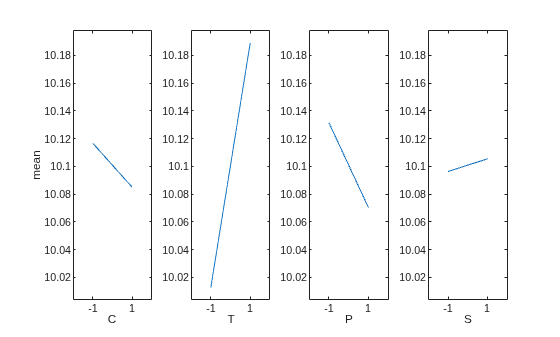
The plot indicates that the mean response is highly sensitive to the temperature setting and less sensitive to the other factor settings.
Create an interaction plot.
figure
interactionplot(y1,D1,VarNames=factorLabels,Full=false)
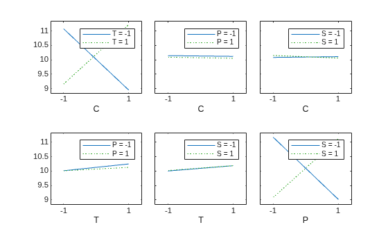
The plot indicates that the response is also sensitive to two-factor interactions. However, because two-factor interactions are confounded with each other in a resolution IV design, you need a full factorial design experiment to determine whether factors C and T or factors S and P are interacting.
Repeat the experiment by creating a full factorial design. Display the size of the design table.
dFull = fullFactorialDOE(4,FactorNames=factorLabels);
D2 = table2array(dFull.Design);
size(D2)
ans = 1×2

    16     4
The full factorial design contains = 16 runs. Load the simulated response data y2 from reaction2.mat.
load reaction2.matCreate an interaction plot.
figure
interactionplot(y2,D2,VarNames=factorLabels,Full=false)
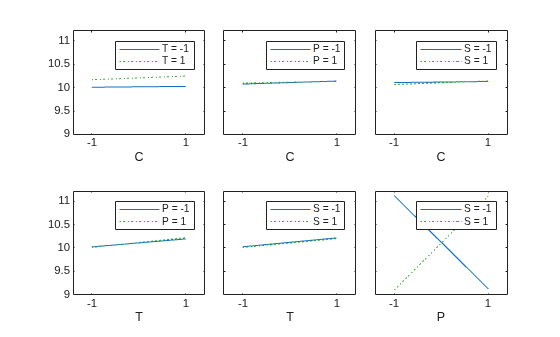
Because the full factorial design does not confound any interactions, the plot indicates that the mean response depends mainly on T and the interaction between S and P.

