plotComparisons

Interactive plot of multiple comparisons of means for analysis of variance (ANOVA)

Since R2022b

Syntax

plotComparisons(aov)

plotComparisons(aov,factors)

plotComparisons(ax,___)

plotComparisons(___,Name=Value)

f = plotComparisons(___)

Description

plotComparisons(aov) creates an interactive plot of the mean responses for each value of the factor in a one-way anova object with comparison intervals.

To a close approximation, the difference between two mean estimates is statistically significant if their comparison intervals are disjoint, and is not statistically significant if their comparison intervals overlap. You can click an estimate to display its mean and comparison interval in blue, statistically different means and comparison intervals in red, and statistically similar means and comparison intervals in gray.

plotComparisons(aov,factors) groups the response data by the values of the factors listed in factors for a one-, two-, or N-way ANOVA.

plotComparisons(ax,___) plots into the axes ax using any of the input argument combinations in the previous syntaxes.

plotComparisons(___,Name=Value) specifies additional options using one or more name-value arguments. For example, you can specify the confidence level for the bounds of the comparison interval.

f = plotComparisons(___) returns a Figure object f. Use f to query or modify properties of the figure after it is created.

Examples

Compare Group Means of One-Way ANOVA

Load popcorn yield data.

load popcorn.mat

The columns of the 6-by-3 matrix popcorn contain popcorn yield observations in cups for the brands Gourmet, National, and Generic, respectively.

Perform a one-way ANOVA to test the null hypothesis that the mean yields are the same across the three brands. Use the function repmat to create a string vector containing factor values for the brand.

factors = [repmat("Gourmet",6,1); repmat("National",6,1); repmat("Generic",6,1)];
aov = anova(factors,popcorn(:),"FactorNames","Brand")

aov = 
1-way anova, constrained (Type III) sums of squares.

Y ~ 1 + Brand

             SumOfSquares    DF    MeanSquares     F        pValue  
             ____________    __    ___________    ____    __________

    Brand       15.75         2        7.875      18.9    7.9603e-05
    Error        6.25        15      0.41667                        
    Total          22        17                                     


  Properties, Methods

aov is an anova object that contains the results of the one-way ANOVA.

The small p-value for Brand indicates that the null hypothesis can be rejected at the 99% confidence level. Enough evidence exists to conclude that at least one brand has a statistically significant difference in mean popcorn yield. You can view this difference by plotting the group means with comparison intervals.

plotComparisons(aov);

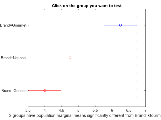
The figure shows the Gourmet comparison interval in blue and the comparison intervals of National and Generic in red. The colors indicate that Gourmet is statistically different from Generic and National.

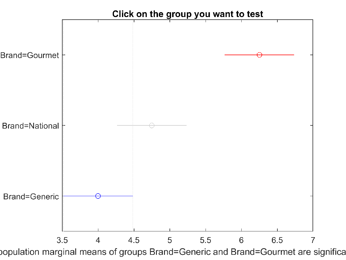
Click on the mean of Generic. The plot now shows the Generic comparison interval in blue, the National comparison interval in gray, and the Gourmet comparison interval in red. The colors indicate that the difference in the mean popcorn yields of Generic and National is not statistically significant.

Input Arguments

aov — Analysis of variance results

anova object

Analysis of variance results, specified as an anova object. The properties of aov contain the factors and response data used by plotComparisons to compute the difference in means.

factors — Factors used to group response data

string vector | cell array of character vectors

Factors used to group the response data, specified as a string vector or cell array of character vectors. The plotComparisons function groups the response data by the combinations of values for the factors in factors. The factors argument must be one or more of the names in aov.FactorNames.

Example: ["g1","g2"]

Data Types: string | cell

ax — Target axes

Axes object

Target axes, specified as an Axes object. If you do not specify the axes, then plotComparisons uses the current axes (gca).

Name-Value Arguments

Specify optional pairs of arguments as Name1=Value1,...,NameN=ValueN, where Name is the argument name and Value is the corresponding value. Name-value arguments must appear after other arguments, but the order of the pairs does not matter.

Example: Alpha=0.01,CriticalValueType="dunnett",Approximate=true sets the significance level of the confidence intervals to 0.01 and uses an approximation of Dunnett's critical value to calculate the p-values for the null hypothesis that group means are not significantly different.

Alpha — Significance level

single | double

Significance level for the comparison intervals, specified as a single or double between 0 and 1. The confidence level of the comparison intervals is the probability that the difference between two mean estimates with overlapping intervals is not statistically significant. The value of Alpha is given by the formula $$100(1-\alpha )\%$$. The default value for Alpha is 0.05.

Example: Alpha=0.01

Data Types: single | double

CriticalValueType — Critical value type

"tukey-kramer" (default) | "hsd" | "dunn-sidak" | "bonferroni" | "scheffe" | "dunnett" | "lsd"

Critical value type used by the plotComparisons function to calculate p-values, specified as one of the options in the following table. Each option specifies the statistical test that plotComparisons uses to calculate the critical value.

Option	Statistical Test
"tukey-kramer" (default)	Tukey-Kramer test
"hsd"	Honestly Significant Difference test — Same as "tukey-kramer"
"dunn-sidak"	Dunn-Sidak correction
"bonferroni"	Bonferroni correction
"scheffe"	Scheffe test
"dunnett"	Dunnett's test — Can be used only when aov is a one-way anova object or when a single factor is specified in factors. For Dunnett's test, the control group is selected in the generated plot and cannot be changed.
"lsd"	Stands for Least Significant Difference and uses the critical value for a plain t-test. This option does not protect against the multiple comparisons problem unless it follows a preliminary overall test such as an F-test.

Example: CriticalValueType="dunn-sidak"

Data Types: char | string

Approximate — Indicator to compute Dunnett critical value approximately

true or 1 | false or 0

Indicator to compute the Dunnett critical value approximately, specified as a numeric or logical 1 (true) or 0 (false). You can compute the Dunnett critical value approximately for speed. The default for Approximate is true for an N-way ANOVA with N greater than two, and false otherwise. This argument is valid only when CriticalValueType is "dunnett".

Example: Approximate=true

Data Types: logical

ControlGroup — Index of control group factor value

1 (default) | positive integer

Index of the control group factor value for Dunnett's test, specified as a positive integer. Factor values are indexed by the order in which they appear in aov.ExpandedFactorNames. This argument is valid only when CriticalValueType is "dunnett".

Example: ControlGroup=3

Data Types: single | double

Output Arguments

f — Target figure

Figure object

Target figure, returned as a Figure object. Use f to query or modify properties of the figure after it is created. For a full list of figure properties, see Figure Properties.

References

[1] Hochberg, Y., and A. C. Tamhane. Multiple Comparison Procedures. Hoboken, NJ: John Wiley & Sons, 1987.

[2] Milliken, G. A., and D. E. Johnson. Analysis of Messy Data, Volume I: Designed Experiments. Boca Raton, FL: Chapman & Hall/CRC Press, 1992.

[3] Searle, S. R., F. M. Speed, and G. A. Milliken. “Population marginal means in the linear model: an alternative to least-squares means.” American Statistician. 1980, pp. 216–221.

[4] Dunnett, Charles W. “A Multiple Comparison Procedure for Comparing Several Treatments with a Control.” Journal of the American Statistical Association, vol. 50, no. 272, Dec. 1955, pp. 1096–121.

[5] Krishnaiah, Paruchuri R., and J. V. Armitage. "Tables for multivariate t distribution." Sankhyā: The Indian Journal of Statistics, Series B (1966): 31-56.

Version History

Introduced in R2022b