Nonlinear Reluctance

Linear or nonlinear reluctance with optional hysteresis

• 

Libraries:
Simscape / Electrical / Passive

Description

The Nonlinear Reluctance block models linear or nonlinear reluctance with optional magnetic hysteresis. Use this block to model custom inductances and build transformer models. To connect this block to your electrical network, use a Winding block to represent the interface between the electrical and magnetic domains.

To define the geometry for the part of the magnetic network that you are modeling, use the Effective length and Effective cross-sectional area parameters. The block uses this geometry information to map B and H to the magnetomotive force and magnetic flux, which are the Through and Across variables in the magnetic domain. Choose how to parameterize the B-H curve using the Parameterized by parameter.

Equations for Linear Reluctance Parameterization

The equations for the linear reluctance parameterization are

$$B= {\mu }_0{\mu }_{r}H$$

$mmf=l_{eff}H$

$\phi =s_{eff}B$

where:

• B is the flux density.

• μ₀ is the permeability in a vacuum.

• μ_r is the relative magnetic permeability.

• H is the field strength.

• mmf is the magnetomotive force (mmf) across the component.

• l_eff is the effective length of the section being modeled.

• φ is the magnetic flux.

• s_eff is the effective cross-sectional area of the section being modeled.

Equations for Reluctance with Single Saturation Point Parameterization

This parameterization models a switch-linear reluctance. In the unsaturated state, the material has a specified relative magnetic permeability. In the saturated state, the relative permeability is 𝜇₀.

The equations for reluctance with single saturation point are

$mmf=l_{eff}H$

$\phi =s_{eff}B$

$mmf=R\phi$

If $B<B_{sat}$,

$B= {\mu }_0{\mu }_{r\_unsat}H.$

Otherwise,

$B=B_{sat}+ {\mu }_0(H-\frac{B_{sat}}{{\mu }_0{\mu }_{r\_unsat}})$

where:

• mmf is the magnetomotive force (mmf) across the component.

• l_eff is the effective length of the section being modeled.

• H is the field strength.

• φ is magnetic flux.

• s_eff is the effective cross-sectional area of the section being modeled.

• B is the flux density.

• B_sat is the flux density at saturation.

• R_sat is the magnetic reluctance at saturation.

• μ₀ is the permeability in a vacuum.

• μ_r is the relative magnetic permeability.

• μ_{r_unsat} is the unsaturated relative magnetic permeability.

Reluctance (B-H Curve)

To model reluctance without hysteresis by tabulating the B-H curve, set the Parameterized by parameter to Reluctance (B-H curve).

Equations for Reluctance with Hysteresis Parameterization

These equations define the flux density and magnetomotive force,

$$B={\phi /s}_{eff}$$

$$mmf=l_{eff}H$$

where:

• B is the magnetic flux density induced in the core.

• φ is the magnetic flux.

• s_eff is the value of the Effective cross-sectional area parameter.

• mmf is the magnetomotive force (mmf) across the component.

• l_eff is the value of the Effective length parameter.

• H is the total field strength.

This equation relates B and H to the total magnetization of the core M,

$$B={\mu }_0\left(H+M\right),$$

where μ₀ is the magnetic permeability of a vacuum.

The magnetization acts to increase the magnetic flux density, and its value depends on both the current value and the history of the field strength. The block uses the Jiles-Atherton [1, 2] equations to determine M at any given time. This figure shows a typical plot of the resulting relationship between B and H.

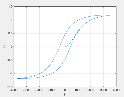
As the field strength increases from H = 0, the plot initially follows an ascending hysteresis curve. At the saturation point, further increases in field intensity no longer cause significant increases in magnetic flux.

As you reduce the magnetic field strength from the saturation point, the plot follows a descending hysteresis curve. The difference between ascending and descending curves is due to the dependence of M on the trajectory history. Physically, the behavior corresponds to magnetic dipoles in the core aligning as the field strength increases, but not then fully recovering to their original position as field strength decreases.

The starting point for the Jiles-Atherton equation is the split of the magnetization effect into two parts, one part that is purely a function of effective field strength H_eff and another, irreversible part that depends on history. This equation defines the relative contributions of the anhysteretic magnetisation M_an and the irreversible magnetization M_irr to the total magnetization M,

$$M=c{M}_{an}+\left(1-c\right)M_{irr},$$

where c is the coefficient for reversible magnetization.

This equation relates M_an to the equivalent magnetization H_eff:

$$M_{an}=M_s\left(\coth \left(\frac{H_{eff}}{a}\right)-\frac{a}{H_{eff}}\right).$$

The function defines a saturation curve with limiting values ±M_s, where:

• M_s is the saturation magnetization.

• a is the anhysteretic magnetization coefficient, which determines the point of saturation. It approximately describes the average of the two hysteretic curves.

In the Nonlinear Reluctance block mask, you provide values for $$d{M}_{an}/d{H}_{eff}$$ when H_eff = 0 and a point [H₁, B₁] on the anhysteretic B-H curve. The block uses these values to determine values for α and M_s.

The Jiles-Atherton model defines the irreversible term by a partial derivative with respect to field strength,

$$\begin{array}{l}\frac{d{M}_{irr}}{dH}=\frac{M_{an}-M_{irr}}{K\delta -\alpha \left(M_{an}-M_{irr}\right)}\\ \delta =\{\begin{array}{ll}1\hfill & \text{if }H\ge 0\hfill \\ -1\hfill & \text{if }H<0\hfill \end{array}\end{array}$$

where:

• K is the bulk coupling coefficient, which shapes the irreversible characteristic.

• α is the inter-domain coupling factor.

Comparison of the equation with a standard first-order differential equation reveals that as you change the total field strength H, the irreversible term M_irr attempts to track the reversible term M_an, but with a variable tracking gain of $$1/\left(K\delta -\alpha \left(M_{an}-M_{irr}\right)\right)$$. The tracking error acts to create the hysteresis at the points where δ changes sign.

This equation defines the effective field strength of an anhysteretic curve,

$$H_{eff}=H+\alpha M.$$

The value of α affects the shape of the hysteresis curve. Larger values act to increase the B-axis intercepts. However, the stability term $$K\delta -\alpha \left(M_{an}-M_{irr}\right)$$ must be positive for δ > 0 and negative for δ < 0. There are therefore limits on the values of α that you can provide. A typical maximum value is of the order 1e-3.

Note

You can also use the Magnetic Core block to model a magnetic core that exhibits nonlinear reluctance and hysteresis. Both blocks use the Jiles-Atherton model to determine the relationship between B, H, and M. However, the Magnetic Core block gives you additional options:

• In addition to specifying the Jiles-Atherton parameters directly, you can parameterize the B-H curve using these options:

  • Specify the magnitude of the B and H intercepts and the magnitude of B and H at the saturation point.

  • Tabulate the ascending or descending B-H curves.

• You can model eddy losses and thermal effects.

Procedure for Finding Approximate Values for Jiles-Atherton (JA) Equation Coefficients

You can determine representative values for the equation coefficients using this procedure:

1. Provide a value for the Anhysteretic B-H gradient when H is zero parameter ($$d{M}_{an}/d{H}_{eff}$$ when H_eff = 0) and a data point [H₁, B₁] on the anhysteretic B-H curve. From these values, the block initialization determines values for α and M_s.

2. Set the Coefficient for reversible magnetization, c parameter to achieve correct initial B-H gradient when starting a simulation from [H B] = [0 0]. The value of c is approximately the ratio of this initial gradient to the Anhysteretic B-H gradient when H is zero. The value of c must be greater than 0 and less than 1.

3. Set the Bulk coupling coefficient, K parameter to the approximate magnitude of H when B = 0 on the ascending hysteresis curve.

4. Start with a very small value for the Inter-domain coupling factor, alpha parameter, and gradually increase it to tune the value of B when crossing the H = 0 line. A typical value is in the range of 1e-4 to 1e-3. Values that are too large cause the gradient of the B-H curve to tend to infinity, which is nonphysical and generates a run-time assertion error.

To get a good match against a predefined B-H curve, iterate on these four steps.

Variables

To set the priority and initial target values for the block variables before simulation, use the Initial Targets section in the block dialog box or Property Inspector. For more information, see Set Priority and Initial Target for Block Variables.

Use nominal values to specify the expected magnitude of a variable in a model. Using system scaling based on nominal values increases the simulation robustness. Nominal values can come from different sources. One of these sources is the Nominal Values section in the block dialog box or Property Inspector. For more information, see System Scaling by Nominal Values.

Examples

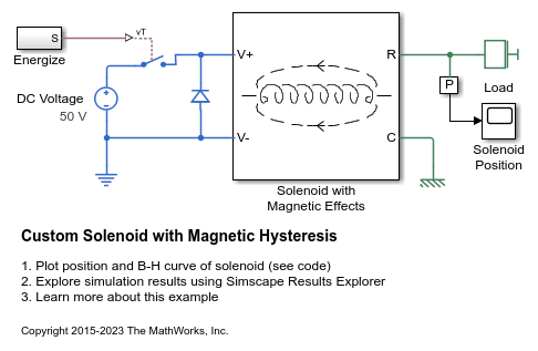
Custom Solenoid with Magnetic Hysteresis

A limited travel solenoid with return spring. Magnetic hysteresis is modeled using the Reluctance with Hysteresis library block.

• Open Model

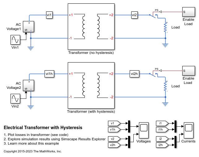
Electrical Transformer with Hysteresis

Model a custom transformer that exhibits hysteresis by using the Non Linear Reluctance block in a magnetic circuit. The transformer is rated for a 50W load and steps down from 120V to 12V rms. The magnetizing resistance Rm is modeled in the magnetic domain using an Eddy Loss block.

• Open Model

Inductor with Hysteresis

How modifying the equation coefficients of the Jiles-Atherton magnetic hysteresis equations affects the resulting B-H curve. The simulation parameters are configured to run four complete AC cycles with initial field strength (H) and magnetic flux density (B) both set to zero.

• Open Model

Ports

Conserving

N — North terminal

magnetic

Magnetic conserving port associated with the north terminal.

S — South terminal

magnetic

Magnetic conserving port associated with the south terminal.

Parameters

To edit block parameters interactively, use the Property Inspector. From the Simulink^® Toolstrip, on the Simulation tab, in the Prepare gallery, select Property Inspector.

Main

Effective length — Effective core length

0.032 m (default) | positive finite scalar

Effective core length. This parameter represents the average length of the magnetic path around the core.

Effective cross-sectional area — Effective core cross-sectional area

1.6e-5 m^2 (default) | positive finite scalar

Effective core cross-sectional area. This parameter represents the average area of the magnetic path around the core.

Averaging period for power logging — Excitation period used for averaging

0 s (default) | scalar

Averaging period for the hysteresis losses calculation. These losses are proportional to the area enclosed by the B-H trajectory. If you excite the block at a known, fixed frequency, you can set this value to the corresponding excitation period to calculate the hysteresis loss. The block logs the hysteresis loss once per AC cycle in the power_dissipated variable in the logged simulation data. If you are using a fixed-step solver, this value must be an integer multiple of the simulation step size.

If you do not excite the block at a known, fixed frequency, set this parameter to 0. The block sets the power_dissipated variable in the logged simulation data to 0. You can calculate the actual hysteresis loss by post-processing the power_instantaneous variable in the logged simulation data.

Dependencies

To enable this parameter, in the B-H Curve settings, set the Parameterized by parameter to Nonlinear reluctance with hysteresis (JA model).

B-H Curve

Parameterized by — Parameterization method

Reluctance (B-H curve) (default) | Linear reluctance | Reluctance with single saturation point | Nonlinear reluctance with hysteresis (JA model)

Parameterization method that you use to describe the B-H curve. Choose one of these options:

• Reluctance (B-H curve) — Model reluctance without hysteresis by tabulating the B-H curve.

• Linear reluctance — Model linear reluctance by specifying the relative magnetic permeability.

• Reluctance with single saturation point — Model switch-linear reluctance without hysteresis, by specifying the unsaturated relative magnetic permeability and magnetic flux at saturation.

• Nonlinear reluctance with hysteresis (JA model) — Model nonlinear reluctance with hysteresis by specifying the Jiles-Atherton parameters.

Selecting a parameterization method enables related parameters in the B-H Curve settings. If you set this parameter to Nonlinear reluctance with hysteresis (JA model), you enable the Averaging period for power logging parameter in the Main settings.

Relative magnetic permeability — Relative magnetic permeability

5000 (default) | positive finite scalar

Relative magnetic permeability.

Dependencies

To enable this parameter, set Parameterized by to Linear reluctance.

Unsaturated relative magnetic permeability — Relative magnetic permeability

5000 (default) | scalar

Relative magnetic permeability for an unsaturated inductor.

Dependencies

To enable this parameter, set Parameterized by to Reluctance with single saturation point.

Magnetic flux density at saturation — Magnetic flux density at saturation

1.5 T (default) | positive finite scalar

Magnetic flux density for a saturated inductor.

Dependencies

To enable this parameter, set Parameterized by to Reluctance with single saturation point.

Magnetic field strength vector, H — Magnetic field strength

[0, 200, 400, 600, 800, 1000] A/m (default) | vector

Magnetic field strength H, specified as a vector with the same number of elements as the magnetic flux density B. These vectors must start with zero and increase monotonically.

Dependencies

To enable this parameter, set Parameterized by to Reluctance (B-H curve).

Magnetic flux density vector, B — Magnetic flux density

[0, 1.25, 1.35, 1.44, 1.48, 1.49] T (default) | vector

Magnetic flux density B, specified as a vector with the same number of elements as the magnetic field strength vector H. These vectors must start with zero and increase monotonically.

Dependencies

To enable this parameter, set Parameterized by to Reluctance (B-H curve).

Interpolation method — Interpolation method

Linear (default) | Smooth

Interpolation method that the block uses to determine B and H at intermediate points that you do not specify. Choose one of these options:

• Linear — Prioritize performance by using a linear function.

• Smooth — Prioritize accuracy by producing a continuous curve with continuous first-order derivatives.

Dependencies

To enable this parameter, set Parameterized by to Reluctance (B-H curve).

Anhysteretic B-H gradient when H is zero — Gradient of anhysteretic B-H curve around zero field strength

0.0063 m*T/A (default) | scalar

Gradient of the anhysteretic B-H curve around zero field strength. Set this parameter to the average gradient of the ascending and descending hysteresis curves.

Dependencies

To enable this parameter, set Parameterized by to Nonlinear reluctance with hysteresis (JA model).

Flux density point on anhysteretic B-H curve — Flux density of the point for field strength measurement

1.49 T (default) | scalar

Flux density of the point for field strength measurement. You must specify a point on the anhysteretic curve by providing its flux density value. To obtain accurate results, pick a point at high field strength where the ascending and descending hysteresis curves align.

Dependencies

To enable this parameter, set Parameterized by to Nonlinear reluctance with hysteresis (JA model).

Corresponding field strength — Field strength at measurement point

1000 A/m (default) | scalar

Field strength that corresponds to the point that you define using the Flux density point on anhysteretic B-H curve parameter.

Dependencies

To enable this parameter, set Parameterized by to Nonlinear reluctance with hysteresis (JA model).

Coefficient for reversible magnetization, c — Coefficient for reversible magnetization

0.1 (default) | scalar in the range [0,1]

Coefficient for reversible magnetization in the Jiles-Atherton equations, c. This parameter represents the proportion of the magnetization that you can reverse.

Dependencies

To enable this parameter, set Parameterized by to Nonlinear reluctance with hysteresis (JA model).

Bulk coupling coefficient, K — Jiles-Atherton equations parameter

200 A/m (default) | finite positive scalar

Bulk coupling coefficient in the Jiles-Atherton equations, K. This parameter primarily controls the field strength magnitude at which the B-H curve crosses the zero flux density line.

Dependencies

To enable this parameter, set Parameterized by to Nonlinear reluctance with hysteresis (JA model).

Inter-domain coupling factor, alpha — Jiles-Atherton equations parameter

0.0001 (default) | scalar

Inter-domain coupling factor in the Jiles-Atherton equations, α. This parameter primarily affects the points at which the B-H curves intersect the zero field strength line. Typical values are in the range of 1e-4 to 1e-3.

Dependencies

To enable this parameter, set Parameterized by to Nonlinear reluctance with hysteresis (JA model).

References

[1] Jiles, D. C. and D. L. Atherton. "Theory of ferromagnetic hysteresis." Journal of Magnetism and Magnetic Materials 61, no. 1–2 (September 1986): 48–60. https://doi.org/10.1016/0304-8853(86)90066-1.

[2] Jiles, D. C. and D. L. Atherton. “Ferromagnetic hysteresis.” IEEE^® Transactions on Magnetics 19, no. 5 (September 1983): 2183–2185. https://doi.org/10.1109/TMAG.1983.1062594.

Extended Capabilities

C/C++ Code Generation
Generate C and C++ code using Simulink® Coder™.

Version History

Introduced in R2017b