Top-Level Model Coverage Report

If you analyze coverage for your model using the Run button, Simulink^® Coverage™ creates a model coverage report for the specified model named model_name_cov.html. The Simulink Coverage report opens in the Coverage Details pane of the Simulink window.

For more information about analyzing coverage, see Generate Coverage Results for Models.

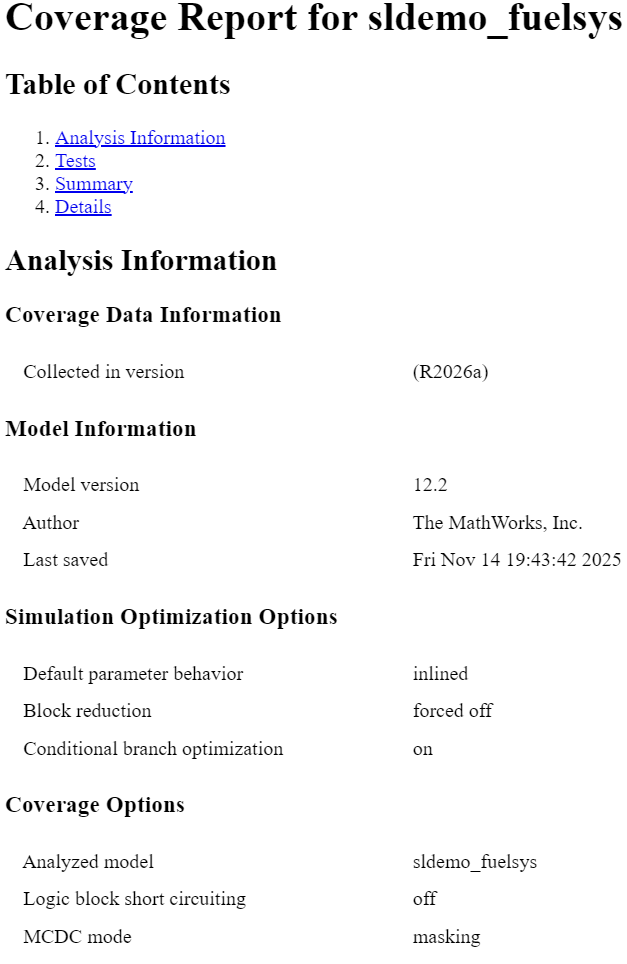
Analysis Information

The analysis information section contains basic information about the model being analyzed:

• Coverage Data Information

• Model Information

• Harness Information (appears if you record coverage from a Simulink Test™ harness)

• Simulation Optimization Options

• Coverage Options

Objects Filtered from Coverage Analysis

The Objects Filtered from Coverage Analysis section lists the objects in the model that were filtered from coverage recording and the rationale specified for filtering them. If the filter rule specifies that all blocks of a certain type be filtered, the coverage report lists all of those blocks here.

In the following image, an exclusion rule filters a Product block named Product. The coverage report displays the name, full path and file name of the coverage filter. It also displays the filter description, list of blocks, and the rationales used to filter them. In the table of filtered model objects, the table also links to the block. Clicking the link navigates to the block within the model and highlights it with a blue border. Clicking the filter name or the link in the rationale column opens the Coverage Results Explorer to the Filter Editor pane and displays the filter rule.

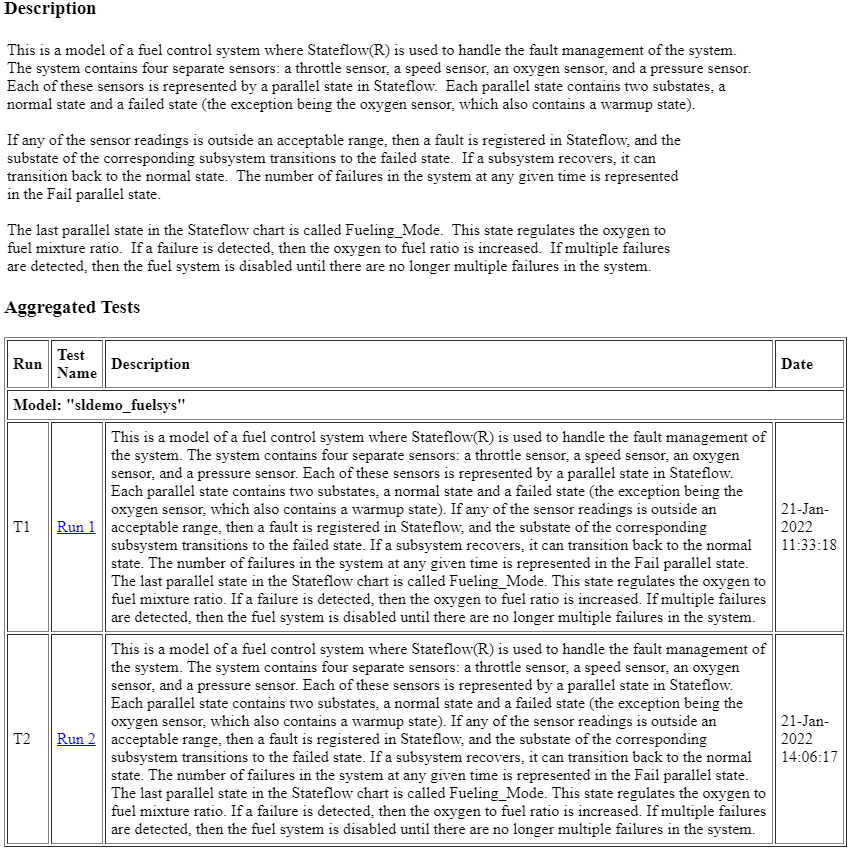
Aggregated Tests

The aggregated tests section appears if you:

• Record aggregated coverage results for at least two test cases through the Simulink Test Manager and produce a coverage report for the aggregated results, or

• Produce a coverage report for cumulative coverage results in the Results Explorer.

If you run test cases through the Simulink Test Manager, the aggregated tests section links to the associated test cases in the Simulink Test Manager.

If you aggregate test case results through the Results Explorer, the aggregated tests section links to the corresponding cvdata node in the Results Explorer.

For each run in the aggregated tests section, there is a link to the corresponding results in the Simulink Test Manager or the Results Explorer.

Aggregated Unit Tests

If you record coverage for one or more subsystem harnesses, the Aggregated Tests section lists each unit test run, and the Description section displays the description given to the aggregated coverage data. You can see and edit this description by going to the Coverage Results Explorer and clicking Current Cumulative Data.

Each unit under test receives an ordinal number n, and each test for a unit under test receives an ordinal number m in the style Un.m.

Coverage Summary

The coverage summary has two subsections:

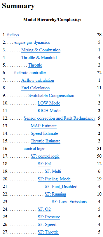
• Tests — The simulation start and stop time of each test case and any setup commands that preceded the simulation. The heading for each test case includes any test case label specified using the cvtest command. This section only shows when the report does not contain an Aggregated Tests section.

• Summary — Summaries of the subsystem results. To see detailed results for a specific subsystem, in the Summary subsection, click the subsystem name.

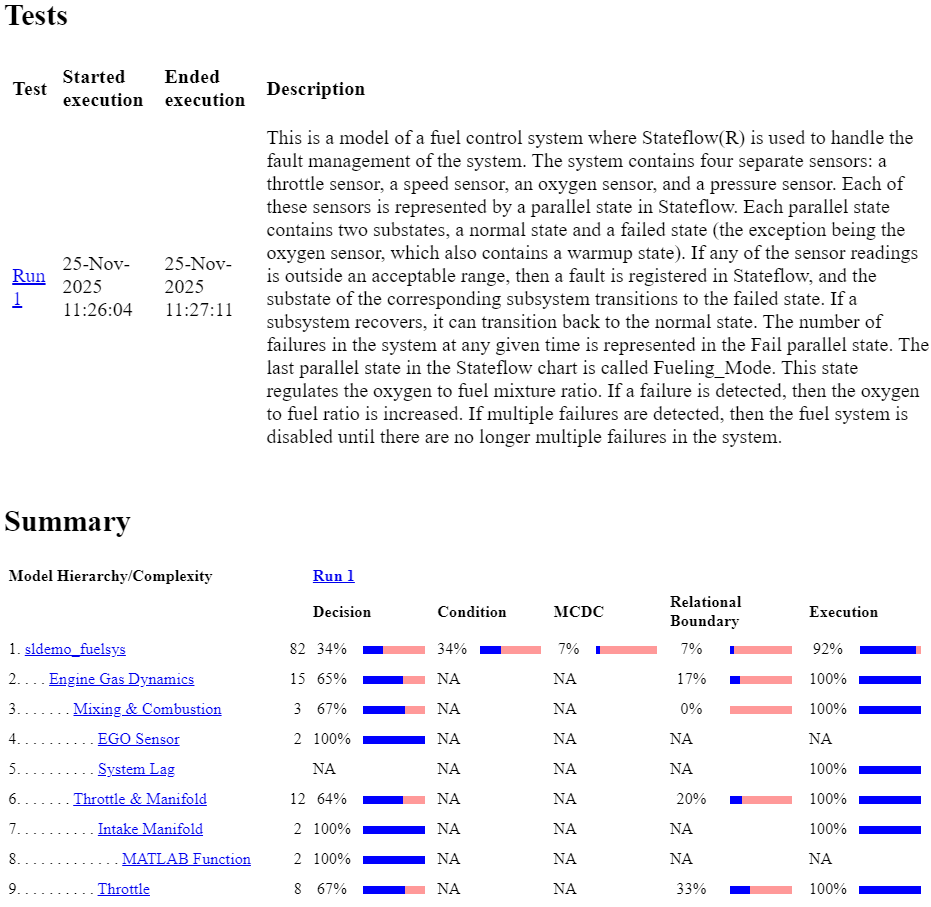
The Summary section contains a column for each requested coverage metric, even for metrics that are not applicable to the model or model objects analyzed. For example, in the sldemo_fuelsys model, if you select the Objectives and constraints coverage metric, you get columns titled Test Objective, Proof Objective, Test Condition, and Proof Assumption, even though the model does not contain blocks that Simulink Coverage can analyze for these metrics.

Missing Model Coverage Analysis

The Missing Model Coverage Analysis section appears when your model has missing coverage.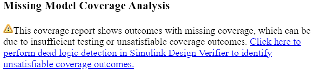

Click the link to open the Perform Dead Logic Detection dialog box, which allows you to run dead logic detection analysis using Simulink Design Verifier™.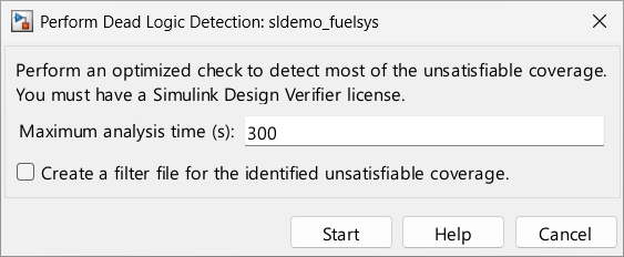

In the Perform Dead Logic Detection dialog box, you can change the maximum analysis time and choose whether to create coverage justification rules for the coverage outcomes that the analysis identifies as dead logic.

Note

When you run dead logic detection using this dialog box, Simulink Design Verifier ignores the value of the Run exhaustive analysis (Simulink Design Verifier) parameter, and does not run exhaustive analysis.

After running dead logic detection analysis, you should verify that the identified logic is unreachable and decide what to do about it. If you select the Create a filter file for the identified unsatisfiable coverage option, you should decide whether to keep those justification rules applied to the coverage results or remove them and address the dead logic another way, such as by editing the model to remove it.

Details

The Details section reports the detailed model coverage results. Each section of the detailed report summarizes the results for the metrics that test each object in the model:

• Blocks Eliminated from Coverage Analysis

• Model Details

• Subsystem Details

• Block Details

• Chart Details

• Coverage Details for MATLAB Functions and Simulink Design Verifier Functions

• Requirement Testing Details

You can also access a model element details subsection by clicking that block or other model element.

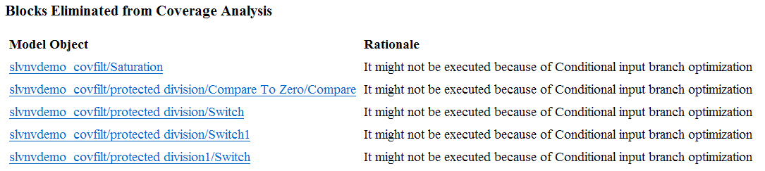
Blocks Eliminated from Coverage Analysis

The Blocks Eliminated from Coverage Analysis section lists each block that might be missing coverage or were not included in coverage analysis due to optimizations such as conditional input branch optimization or block reduction. For more information, see Simulink Optimizations and Model Coverage.

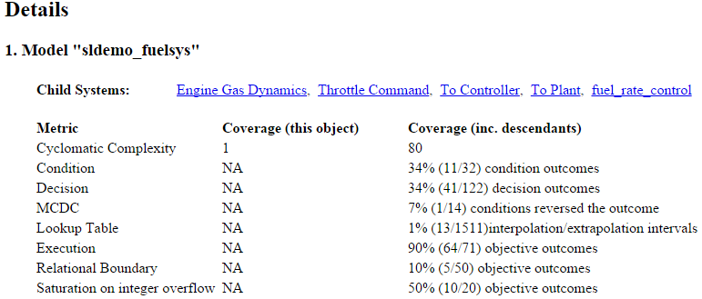
Model Details

The Details section contains a results summary for the model as a whole, followed by a list of elements. Click the model element name to see its coverage results.

The following graphic shows the Details section for the sldemo_fuelsys example model.

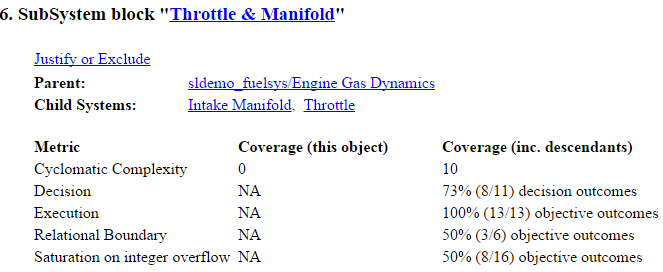
Subsystem Details

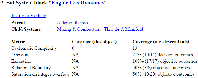
Each subsystem Details section contains a summary of the test coverage results for the subsystem and a list of the subsystems it contains. The overview is followed by sections for blocks, charts, and MATLAB^® functions, one for each object that contains a decision point in the subsystem.

The following graphic shows the coverage results for the Engine Gas Dynamics subsystem in the sldemo_fuelsys example model.

Block Details

The following image shows decision coverage results for the MinMax block in the Engine Gas Dynamics/Mixing & Combustion subsystem in the sldemo_fuelsys example model.

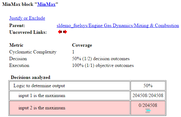
The Uncovered Links element first appears in the Block Details section of the first block in the model hierarchy that does not achieve 100% coverage. The first Uncovered Links element has an arrow that links to the Block Details section in the report of the next block that does not achieve 100% coverage.

Subsequent blocks that do not achieve 100% coverage have links to the Block Details sections in the report of the previous and next blocks that do not achieve 100% coverage.

The decisions analyzed table displays each possible outcome of each decision in a block, as well as the number of time steps each outcome occurs during the simulation. In this case, the MinMax block decision is true for 204,508 time steps out of a total of 204,508 time steps that the decision is evaluated, and is not false for any time step. For more information about the coverage tables, see the sections for each metric, such as Decisions Analyzed.

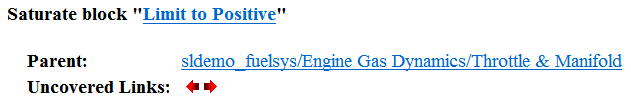
Chart Details

The following graphic shows the coverage results for the Stateflow^® chart control_logic in the sldemo_fuelsys example model.

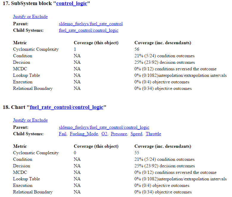
For more information about model coverage reports for Stateflow charts and their objects, see Model Coverage for Stateflow Charts.

Coverage Details for MATLAB Functions and Simulink Design Verifier Functions

By default, Simulink Coverage records coverage for all MATLAB functions in a model. MATLAB functions are in MATLAB Function blocks, Stateflow charts, or external MATLAB files.

Note

For a detailed example of coverage reports for external MATLAB files, see External MATLAB File Coverage Report.

To record Simulink Design Verifier coverage for sldv.* functions called by MATLAB functions, and any Simulink Design Verifier blocks, select Objectives and Constraints on the Coverage pane of the Configuration Parameters dialog box.

The following example shows coverage details for a MATLAB function, hFcnsInExternalEML, that calls four Simulink Design Verifier functions. In this example, the code for hFcnsInExternalEML resides in an external file.

This example also shows Simulink Design Verifier coverage details for the following functions:

• sldv.assume (Simulink Design Verifier)

• sldv.condition (Simulink Design Verifier)

• sldv.prove (Simulink Design Verifier)

• sldv.test (Simulink Design Verifier)

In the coverage results, code that achieves 100% coverage is green. Code that achieves less than 100% coverage is red.

Coverage for the hFcnsInExternalEML function and the sldv.* calls is:

• Line 1, the function declaration for hFcnsInExternalEMLis green because the simulation executes that function at least once. fcn calls hFcnsInExternalEML 11 times during simulation.

  

  Line 4, sldv.assume(u1 > u2), achieves 0% coverage because u1 > u2 never evaluates to true.

  

• Line 5, sldv.condition(u1 == 0), achieves 100% coverage because u1 == 0 evaluates to true for at least one time step.

  

• Line 6, switch u1, achieves 25% coverage because only one of the four outcomes in the switch statement (case 0) occurs during simulation.

  

• Line 17, sldv.test(y > u1); sldv.test (y == 4) achieves 50% coverage. The first sldv.test call achieves 100% coverage, but the second sldv.test call achieves 0% coverage.

  

For more information about coverage for MATLAB functions, see Model Coverage for MATLAB Functions.

For more information about coverage for Simulink Design Verifier functions, see Objectives and Constraints Coverage.

Requirement Testing Details

If you run at least two test cases in Simulink Test that are linked to requirements in Requirements Toolbox™, the aggregated coverage report details the links between model elements, test cases, and linked requirements.

The Requirement Testing Details section includes:

• Implemented Requirements — Which requirements are linked to the model element.

• Verified by Tests — Which tests verify the requirement.

• Associated Runs — Which runs are associated with each verification test.

For an example of how to trace coverage results to requirements in a coverage report, see Trace Coverage Results to Requirements.

Cyclomatic Complexity in the Model Coverage Report

You can specify that the model coverage report include cyclomatic complexity numbers in two locations in the report:

• The Summary section contains the cyclomatic complexity numbers for each object in the model hierarchy. For a subsystem or Stateflow chart, that number includes the cyclomatic complexity numbers for all their descendants.

  

• The Details sections for each object list the cyclomatic complexity numbers for all individual objects.

  

Execution Analyzed

The Execution analyzed table displays the number of time steps that the block executed during simulation over the total number of time steps in the simulation. The coverage report displays block execution coverage as fully satisfied if the block executed during at least one time step.

In the image, Simulink Coverage reports 100% block execution coverage with the block executing during 204,508 out of 204,508 time steps.

Decisions Analyzed

The Decisions analyzed table lists possible outcomes for a decision and the number of times that an outcome occurred in each test simulation. Outcomes that did not occur are in red highlighted table rows.

The following graphic shows the Decisions analyzed table for the Saturate block in the Throttle & Manifold subsystem of the Engine Gas Dynamics subsystem in the sldemo_fuelsys example model.

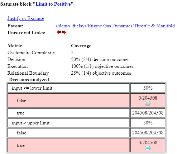
To display and highlight the block in question, click the block name at the top of the section containing the Decisions analyzed table for that block.

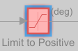
In this case, the decision input >= lower limit is true for 204,508 time steps, and is not false for any time step. The decision input > upper limit is false for 204,508 time steps, and is not true for any time step.

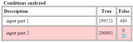
Conditions Analyzed

The Conditions analyzed table lists the number of occurrences of true and false conditions on each input port of the corresponding block.

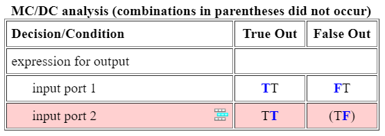
MC/DC Analysis

The MC/DC analysis table lists the expressions that Simulink Coverage analyzes for a given block, followed by rows for each condition. The first row contains the column titles, and the second row displays an expression that represents the logic that Simulink Coverage analyzes for that block. For a single Logical Operator block, this row displays expression for output. If the model contains a cascade of logic blocks or Stateflow charts with conditionalized transitions, the expressions show more detail. For an example of a cascade of logic blocks, see Analyzing MCDC for Cascaded Logic Blocks.

For each row that lists a condition, the first column describes the condition, and the remaining columns display a string where:

• Each character represents the value of an input, where T means true, F means false, and x means the condition was not evaluated due to logical short-circuiting.

• The position of a character in the string corresponds to the position of the condition in the logical expression. For example, in this image, the first character in the string represents the first condition in the logical expression that the block represents, which is input port 1.

• In each row, the condition value of interest is bold and blue.

• Parentheses indicate that the specified combination of inputs did not occur.

To report a row as a satisfied MCDC objective, the value of the condition must affect the output value of the block or expression. For example, consider the MCDC analysis table for a block in the sldemo_fuelsys model, sldemo_fuelsys/fuel_rate_control/airflow_calc/Logic1.

In the model, the Logic1 block is a Logical Operator block with two input ports and one output port. This table explains the MCDC analysis table results for this model:

MC/DC analysis (combinations in parentheses did not occur)			Description
Decision/Condition	True Out	False Out	The True Out column specifies the input values for each row that causes the block to output a true value. The False Out column specifies the values for each row that causes the block to output a false value.
expression for output			If the logic that the block represents is more complex, the first column displays an expression.
input port 1	TT	FT	During simulation, the value of input port 1 changed, while the value of input port 2 did not, and this caused the output value to change. As a result, the MCDC objective for input port 1 is satisfied because this input was shown to independently affect the outcome of the block.
input port 2	TT	(TF)	For input port 2, a value of false did not occur while input port 1 was true. As a result, the MCDC objective for input port 2 is not satisfied.

Because one row is satisfied and one row is not satisfied, the overall MCDC coverage for this block is 50%.

Some model elements achieve less MCDC coverage depending on the MCDC definition used during analysis. For more information about how the MCDC definition affects the coverage results, see Modified Condition and Decision Coverage (MCDC) Definitions in Simulink Coverage.

If you select the Treat Simulink logic blocks as short-circuited model configuration parameter, Simulink Coverage does not evaluate short-circuited inputs that occur in Logical Operator blocks. In this situation, the MCDC analysis table displays an x in a condition expression, such as TFxxx, to indicate that a condition was not analyzed due to logical short-circuiting.

If you want to generate code from your model, select the Treat Simulink Logic blocks as short-circuited model configuration parameter so that the MCDC coverage analysis more closely matches the coverage that your test cases achieve when you analyze code coverage on generated code. Most low-level programming languages like C and C++ short circuit logic. Model coverage and code coverage may not report identical numbers. For more information, see Evaluate Differences Between Model and Code Coverage.

Cumulative Coverage

After you record successive coverage results, you can Manage and Aggregate Coverage Results Using the Coverage Results Explorer from within the Coverage Results Explorer. By default, the results of each simulation are saved and recorded cumulatively in the report.

If you select the Show cumulative progress report parameter, the results located in the right-most area in all tables of the cumulative coverage report reflect the running total value. The report is organized so that you can easily compare the additional coverage from the most recent run with the coverage from all prior runs in the session.

A cumulative coverage report contains information about:

• Current Run — The coverage results of the simulation just completed.

• Delta — Percentage of coverage added to the cumulative coverage achieved with the simulation just completed. If the previous simulation's cumulative coverage and the current coverage are nonzero, the delta may be 0 if the new coverage does not add to the cumulative coverage.

• Cumulative — The total coverage collected for the model up to, and including, the simulation just completed.

After running three test cases, the Summary report shows how much additional coverage the third test case achieved and the cumulative coverage achieved for the first two test cases.

The Decisions analyzed table for cumulative coverage contains three columns of data about decision outcomes that represent the current run, the delta since the last run, and the cumulative data, respectively.

The Conditions analyzed table uses column headers #n T and #n F to indicate results for the current run and delta. The table uses Tot T and Tot F for the cumulative results. You can identify the true and false conditions on each input port of the corresponding block for each test case.

The MCDC analysis #n True Out and #n False Out columns show the condition cases for the current run and delta. The Total Out T and Total Out F column show the cumulative results.

Note

You can calculate cumulative coverage for reusable subsystems and Stateflow constructs at the command line. For more information, see Obtain Cumulative Coverage for Reusable Subsystems.

N-Dimensional Lookup Table

The following interactive chart summarizes the extent to which elements of a lookup table are accessed. In this example, two Sine Wave blocks generate x and y indices that access a 2-D Lookup Table block of 10-by-10 elements filled with random values.

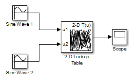
In this model, the lookup table indices are 1, 2,..., 10 in each direction. The Sine Wave 2 block is out of phase with the Sine Wave 1 block by pi/2 radians. This generates x and y numbers for the edge of a circle, which you see when you examine the resulting Lookup Table coverage.

The report contains a two-dimensional table representing the elements of the lookup table. The element indices are represented by the cell border grid lines, which number 10 in each dimension. Areas where the lookup table interpolates between table values are represented by the cell areas. Areas of extrapolation left of element 1 and right of element 10 are represented by cells at the edge of the table, which have no outside border.

Note

The coverage report only generates the Look-up Table Details image for lookup tables that have 400 or fewer interpolation or extrapolation intervals.

The number of values interpolated or extrapolated for each cell (execution counts) during testing is represented by a shade of green assigned to the cell. Each of six levels of green shading and the range of execution counts represented are displayed on one side of the table.

If you click an individual table cell, you see a dialog box that displays the index location of the cell and the exact number of execution counts generated for it during testing. The following example shows the contents of a color-shaded cell on the right edge of the circle.

The selected cell is outlined in red. You can also click the extrapolation cells on the edge of the table.

A bold grid line indicates that at least one block input equal to its exact index value occurred during the simulation. Click the border to display the exact number of hits for that index value.

The following example model uses an n-D Lookup Table block of 10-by-10-by-5 elements filled with random values.

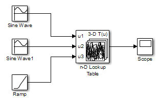
Both the x and y table axes have the indices 1, 2,..., 10. The z axis has the indices 10, 20,..., 50. Lookup table values are accessed with x and y indices that the two Sine Wave blocks generated, in the preceding example, and a z index that a Ramp block generates.

After simulation, you see the following lookup table report.

Instead of a two-dimensional table, the link Force Map Generation displays the following tables:

Lookup table coverage for a three-dimensional lookup table block is reported as a set of two-dimensional tables.

The vertical bars represent the exact z index values: 10, 20, 30, 40, 50. If a vertical bar is bold, this indicates that at least one block input was equal to the exact index value it represents during the simulation. Click a bar to get a coverage report for the exact index value that bar represents.

You can report lookup table coverage for lookup tables of any dimension. Coverage for four-dimensional tables is reported as sets of three-dimensional sets, like those in the preceding example. Five-dimensional tables are reported as sets of sets of three-dimensional sets, and so on.

Block Reduction

All model coverage reports indicate the status of the Simulink Block reduction parameter at the beginning of the report. In the following example, you set Force block reduction off.

In the next example, you enabled the Simulink Block reduction parameter, and you did not set Force block reduction off.

Consider the following model where the simulation does not execute the MinMax1 block because there is only one input — In3.

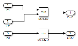
If you set Force block reduction off, the report contains no coverage data for this block because the minimum input to the MinMax1 block is always 1.

If you do not set Force block reduction off, the report contains no coverage data for reduced blocks.

Relational Boundary

On the Coverage Pane of the Configuration Parameters dialog box, if you select the Relational Boundary coverage metric, the software creates a Relational Boundary table in the model coverage report for each model object that is supported for this coverage. The table applies to the explicit or implicit relational operation involved in the model object. For more information, see:

• Relational Boundary Coverage.

• The Relational Boundary column in Model Objects That Receive Coverage.

The tables below show the relational boundary coverage report for the relation input1 <= input2. The appearance of the tables depend on the operand data type.

• Integers

• Fixed point

• Floating point

Integers

If both operands are integers (or if one operand is an integer and the other a Boolean), the table appears as follows.

For a relational operation such as operand_1 <= operand_2:

• The first row states the two operands in the form operand_1 - operand_2.

• The second row states the number of times during the simulation that operand_1 - operand_2 is equal to -1.

• The third row states the number of times during the simulation that operand_1 is equal to operand_2.

• The fourth row states the number of times during the simulation that operand_1 - operand_2 is equal to 1.

Fixed point

If one of the operands has fixed-point type and the other operand is either a fixed point or an integer, the table appears as follows. LSB represents the value of the least significant bit. For more information, see Precision (Fixed-Point Designer). If the two operands have different precision, the smaller value of precision is used.

For a relational operation such as operand_1 <= operand_2:

• The first row states the two operands in the form operand_1 - operand_2.

• The second row states the number of times during the simulation that operand_1 - operand_2 is equal to -LSB.

• The third row states the number of times during the simulation that operand_1 is equal to operand_2.

• The fourth row states the number of times during the simulation that operand_1 - operand_2 is equal to LSB.

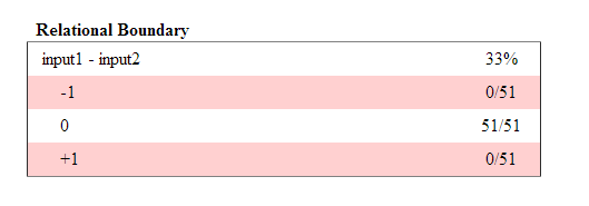
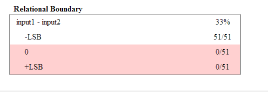
Floating point

If one of the operands has floating-point type, the table appears as follows. tol represents a value computed using the input values and a tolerance that you specify. If you do not specify a tolerance, the default values are used. For more information, see Relational Boundary Coverage.

For a relational operation such as operand_1 <= operand_2:

• The first row states the two operands in the form operand_1 - operand_2.

• The second row states the number of times during the simulation that operand_1 - operand_2 has values in the range [-tol..0].

• The third row states the number of times during the simulation that operand_1 - operand_2 has values in the range (0..tol] during the simulation.

The appearance of this table changes according to the relational operator in the block. Depending on the relational operator, the value of operand_1 - operand_2 equal to 0 is either:

• Excluded from relational boundary coverage.

• Included in the region above the relational boundary.

• Included in the region below the relational boundary.

Relational Operator	Report Format	Explanation
==	[-tol..0)	0 is excluded.
	(0..tol]
!=	[-tol..0)	0 is excluded.
	(0..tol]
<=	[-tol..0]	0 is included in the region below the relational boundary.
	(0..tol]
<	[-tol..0)	0 is included in the region above the relational boundary.
	[0..tol]
>=	[-tol..0)	0 is included in the region above the relational boundary.
	[0..tol]
>	[-tol..0]	0 is included in the region below the relational boundary.
	(0..tol]

0 is included below the relational boundary for <= but above the relational boundary for <. This rule is consistent with decision coverage. For instance:

• For the relation input1 <= input2, the decision is true if input1 is less than or equal to input2. < and = are grouped together. Therefore, 0 lies in the region below the relational boundary.

• For the relation input1 < input2, the decision is true only if input1 is less than input2. > and = are grouped together. Therefore, 0 lies in the region above the relational boundary.

Saturate on Integer Overflow Analysis

On the Coverage Pane of the Configuration Parameters dialog box, if you select the Saturate on integer overflow coverage metric, the software creates a Saturation on Overflow analyzed table in the model coverage report. The software creates the table for each block with the Saturate on integer overflow parameter selected.

The Saturation on Overflow analyzed table lists the number of times a block saturates on integer overflow, indicating a true decision. If the block does not saturate on integer overflow, the table indicates a false decision. Outcomes that do not occur are in red highlighted table rows.

The following graphic shows the Saturation on Overflow analyzed table for the MinMax block in the Mixing & Combustion subsystem of the Engine Gas Dynamics subsystem in the sldemo_fuelsys example model.

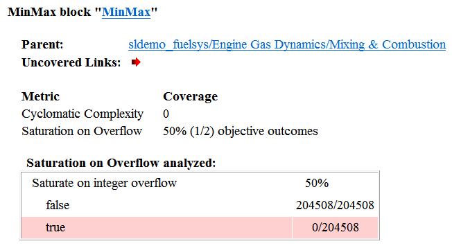
To display and highlight the block in question, click the block name at the top of the section containing the Saturation on Overflow analyzed table for that block.

Signal Range Analysis

If you select the Signal Range coverage metric, the software creates a Signal Range Analysis section at the bottom of the model coverage report. This section lists the maximum and minimum signal values for each output signal in the model measured during simulation.

Access the Signal Range Analysis report quickly with the Signal Ranges link in the nonscrolling region at the top of the model coverage report, as shown below in the sldemo_fuelsys example model report.

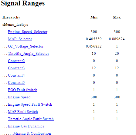
Each block is reported in hierarchical fashion; child blocks appear directly under parent blocks. Each block name in the Signal Ranges report is a link. For example, select the EGO sensor link to display this block highlighted in its native diagram.

Signal Size Coverage for Variable-Dimension Signals

If you select Signal Size, the software creates a Variable Signal Widths section after the Signal Ranges data in the model coverage report. This section lists the maximum and minimum signal sizes for all output ports in the model that have variable-size signals. It also lists the memory that Simulink allocated for that signal, as measured during simulation. This list does not include signals whose size does not vary during simulation.

The following example shows the Variable Signal Widths section in a coverage report. In this example, the Abs block signal size varied from 2 to 5, with an allocation of 5.

Each block is reported in hierarchical fashion; child blocks appear directly under parent blocks. Each block name in the Variable Signal Widths list is a link. Clicking on the link highlights the corresponding block in the Simulink Editor. After the analysis, the variable-size signals have a wider line design.

Simulink Design Verifier Coverage

If you select Objectives and Constraints, the analysis collects coverage data for all Simulink Design Verifier blocks in your model.

For an example of how this works, open the sldvdemo_debounce_testobjblks model.

This model contains two Test Objective blocks:

• The True block defines a property that the signal have a value of 2.

• The Edge block, inside the Masked Objective subsystem, describes the property where the output of the AND block in the Masked Objective subsystem changes from 2 to 1.

The Simulink Design Verifier software analyzes this model and produces a harness model that contains test cases that achieve certain test objectives. To see if the original model achieves those objectives, simulate the harness model and collect model coverage data. The model coverage tool analyzes any decision points or values within an interval that you specify in the Test Objective block.

In this example, the coverage report shows that you achieved 100% coverage of the True block because the signal value was 2 at least once. The signal value was 2 in 6 out of 14 time steps.

The input signal to the Edge block achieved a value of True once out of 14 time steps.