Steady-State Simulation with Projection-Based Trim Optimizer
This example shows how to find a steady-state operating point for a Simscape™ Multibody™ model using the findop function with a projection-based optimizer.
Projection-based optimizers enforce the consistency of the model initial conditions at each evaluation of the objective function or nonlinear constraint function, which can improve trimming results for Simscape models. Using projection-based trim optimizers requires Optimization Toolbox™ software.
Open Model
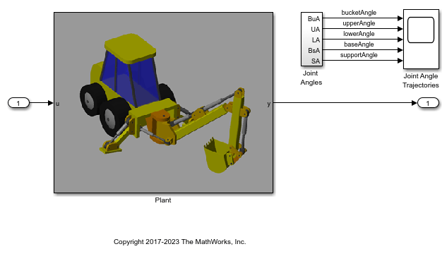
The model for this example is a backhoe system modeled in Simscape Multibody.
Open the Simulink® model.
mdl = "scdbackhoeTRIM";
open_system(mdl)
Define Operating Point Specifications
To define operating point specifications, first create a specification object. The input, output, and state values in ops match the model initial conditions.
opspec = operspec(mdl);
Specify that the model outputs are known values for trimming.
opspec.Outputs(1).Known = true(10,1);
Specify known values for the angles in the backhoe system.
opspec.Outputs(1).y(1) = 0;    % Bucket angle
opspec.Outputs(1).y(3) = 50;   % Upper angle
opspec.Outputs(1).y(5) = -50;  % Lower angle
opspec.Outputs(1).y(7) = 0;    % Base angle
opspec.Outputs(1).y(9) = -45;  % Support angle
For the corresponding angular velocities, the known values are zero, which match the model initial conditions in opspec.
Trim Model
Create an option set for trimming and specify the optimizer type using the OptimizerType option. For this example use the projection-based gradient-descent solver. To view an iterative update of the trimming progress in the Command Window, set the DisplayReport option to "iter".
opt = findopOptions(OptimizerType="graddescent-proj",...
                    DisplayReport="iter");
Specify the maximum number of function evaluations for optimization.
opt.OptimizationOptions.MaxFunEvals = 20000;
Find the steady-state operating point that meets the specifications in opspec. This operation takes several minutes.
op = findop(mdl,opspec,opt);
Optimizing to solve for all desired dx/dt=0, x(k+1)-x(k)=0, and y=ydes.

(Maximum Error)  Block
 ---------------------------------------------------------
(4.50000e+01) scdbackhoeTRIM/Out1
(3.54438e+00) scdbackhoeTRIM/Out1
(2.29753e-01) scdbackhoeTRIM/Out1
(3.84533e-02) scdbackhoeTRIM/Plant/Mounting Assembly/Mounting Base and Support Arms/Support  Arm Right/Revolute Joint  Arm
(9.31533e-03) scdbackhoeTRIM/Plant/Mounting Assembly/Mounting Base and Support Arms/Support  Arm Right/Revolute Joint  Arm
(7.29366e-04) scdbackhoeTRIM/Plant/Mounting Assembly/Mounting Base and Support Arms/Support  Arm Left/Revolute Joint  Arm
(6.64787e-04) scdbackhoeTRIM/Plant/Mounting Assembly/Mounting Base and Support Arms/Support  Arm Left/Revolute Joint  Arm
(8.99706e-05) scdbackhoeTRIM/Plant/Mounting Assembly/Mounting Base and Support Arms/Support  Arm Left/Revolute Joint  Arm
(1.42422e-05) scdbackhoeTRIM/Plant/Mounting Assembly/Mounting Base and Support Arms/Support  Arm Left/Revolute Joint  Arm
(1.42422e-05) scdbackhoeTRIM/Plant/Mounting Assembly/Mounting Base and Support Arms/Support  Arm Left/Revolute Joint  Arm

Operating point search completed successfully using optimization.
Simulate Model
Configure the model to use the computed operating point op as the model initial condition.
set_param(mdl,"LoadExternalInput","on")
set_param(mdl,"ExternalInput","getinputstruct(op)")
set_param(mdl,"LoadInitialState","on")
set_param(mdl,"InitialState","getstatestruct(op)")
Simulate the model.
sim(mdl);
View the joint angle trajectories.
open_system(mdl + "/Joint Angle Trajectories")

The simulation results show that the five angles are trimmed to their expected values. The trajectory can deviate slightly over time due to numerical noise and instability. You can stabilize the angles using feedback controllers.