Model Series RLC Circuit as Implicit State-Space System

R2026b

This example shows how to model a series RLC circuit as an implicit state-space system by using the Descriptor State-Space block.

Conservation laws for physical systems, such as the series RLC circuit, introduce algebraic constraints. Because of the algebraic constraints, these systems are governed by a system of differential-algebraic equations (DAEs).

Directly modeling the DAEs of the series RLC circuit in Simulink™ creates an algebraic loop. By implementing the system in implicit state-space form using the Descriptor State-Space block, you can model the algebraic constraint without an algebraic loop.

Derive RLC Circuit System Equations

Consider this series RLC circuit with a single AC voltage source.

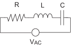
To derive the system of DAEs, start with Kirchhoff's voltage law, which states that the sum of voltages across all components in the loop must be 0.

$$v_{AC}=v_R+v_L+v_C$$

Write the expressions that define the voltages across each component.

$$v_R(t)=i(t)R$$

$$v_L(t)=L\frac{di(t)}{dt}$$

$$v_C(t)=v_C(0)+\frac{1}{C}{\int }_0^{t}i(\tau )d\tau ,$$

where:

• $$i(t)$$ is the current.

• $$R$$ is the resistance of the resistor.

• $$L$$ is the inductance of the inductor.

• $$C$$ is the capacitance of the capacitor.

• $$v_C(0)$$ is the initial condition of the capacitor voltage.

• $$\tau$$ is a dummy variable that represents time.

Replace the terms in the KVL equation with the voltage expressions.

$$v_{AC}(t)=i(t)R+L\frac{di(t)}{dt}+v_C(0)+\frac{1}{C}{\int }_0^{t}i(\tau )d\tau$$

Suppose you want to determine the resistor voltage over time. To solve for the resistor voltage, rearrange the terms in the equation.

$$v_R(t)=v_{AC}(t)-L\frac{di(t)}{dt}-v_C(0)-\frac{1}{C}{\int }_0^{t}i(\tau )d\tau$$

To express the equation in terms of a single variable, replace the inductor and capacitor current terms. Kirchhoff's current law (KCL) states that the sum of all currents at a node must be 0. In the series circuit, each node connects exactly two components, so the current in each component is the same. Replace the current terms with the expression for the resistor current determined by Ohm's law. Assuming the system starts at rest, the initial capacitor voltage is 0. The equation becomes:

$$v_R(t)=v_{AC}(t)-L\frac{d}{dt}\left(\frac{v_R(t)}{R}\right)-\frac{1}{C}{\int }_0^t\frac{v_R(\tau )}{R}d\tau .$$

Model System Equations Directly

Open the model RLCAlgebraicLoop, which implements the equation directly using Gain, Integrator, Derivative, Sine Wave, and Sum blocks.

aloopmdl = "RLCAlgebraicLoop";
open_system(aloopmdl)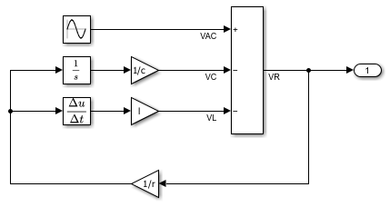

The variables that define the parameter values in the gain blocks are defined in the model workspace. The model simulates a system with a 10$$\Omega$$ resistor, a 1$$\mu H$$ inductor, and a 100$$\mu F$$ capacitor.

Simulate the model. The simulation issues a warning about the algebraic loop.

outaloop = sim(aloopmdl);

Warning: Model '<a href="matlab:open_system ('RLCAlgebraicLoop')">RLCAlgebraicLoop</a>' contains 1 algebraic loops. 
Suggested Actions:
    • Highlight and view information about the algebraic loops in the model using the Simulink.BlockDiagram.getAlgebraicLoops function. - <a href="matlab:Simulink.BlockDiagram.getAlgebraicLoops('RLCAlgebraicLoop');">Open</a>
    • Suppress this diagnostic by setting the 'Algebraic Loop' diagnostic parameter to 'none'. - <a href="matlab:set_param('RLCAlgebraicLoop','AlgebraicLoopMsg', 'none');">Fix</a>

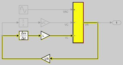
Found algebraic loop that contains: 
RLCAlgebraicLoop/Gain2
RLCAlgebraicLoop/Derivative
RLCAlgebraicLoop/Gain1
RLCAlgebraicLoop/Add (algebraic variable)

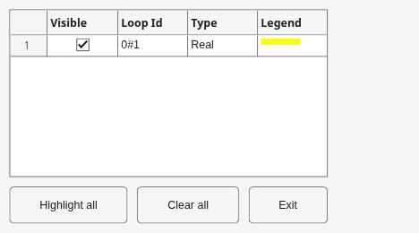
Directly implementing equations is the natural approach to modeling a system in Simulink, but this approach does not always produce the best model. In this case, direct implementation introduces an algebraic loop. To solve the algebraic loop, the simulator invokes the algebraic loop solver, which can slow down simulations. To highlight the loop, use the Simulink.BlockDiagram.getAlgebraicLoops function.

aloop = Simulink.BlockDiagram.getAlgebraicLoops(aloopmdl);

Model Implicit State-Space System Using Descriptor State-Space Block

The Descriptor State-Space block models system dynamics in implicit state-space form:

$$E\underset{}{\overset{\dot{}}{x}}=Ax+Bu$$

$$y=Cx+Du,$$

where:

• The state vector $$x$$ defines the system states, including both dynamic states and algebraic variables.

• The output vector $$y$$ defines the system outputs.

• The input vector $$u$$ defines the system inputs.

• The mass matrix $$E$$ defines state derivative dependencies in the system equations.

• The state matrix $$A$$ defines dependencies between states.

• The input matrix $$B$$ defines dependencies between inputs and states.

• The output matrix $$C$$ defines dependencies between states and outputs.

• The feedthrough matrix $$D$$ defines direct dependencies between inputs and outputs.

The prior derivation produced a single equation with a single variable through substitution. The implicit state-space approach models the system as a system of equations. Each row in the system matrices represents an equation. Each column in the system matrices represents a state or algebraic variable.

To derive the implicit state-space expression of the system:

1. Determine the elements of the state vector. In an implicit system, the state vector contains system states and algebraic variables.

2. Write equations that define relationships among system states and algebraic variables.

3. Define the outputs you want to observe.

4. Construct the system matrices.

For the series RLC circuit, the state vector has five elements: $$v_C$$, $$i_L$$, $$v_R$$, $$v_L$$, and $$i_R$$. $$v_C$$ and $$i_L$$ are dynamic states. The other elements are algebraic variables.

These equations define how the states and algebraic variables relate to each other, expressed with state derivatives on the left and the states and inputs on the right:

$$\frac{d{v}_C}{dt}=\frac{1}{C}{i}_R$$

$$\frac{d{i}_L}{dt}=\frac{1}{L}{v}_L$$

$$0=-v_R+R{i}_L$$

$$0=v_C+v_L+v_R-v_{AC}$$

$$0=i_L-i_R.$$

To observe the resistor voltage as an output, express the output equation as $$y=v_R$$.

The implicit state-space expression of the system becomes:

$$\left(\begin{array}{ccccc}1& 0& 0& 0& 0\\ 0& 1& 0& 0& 0\\ 0& 0& 0& 0& 0\\ 0& 0& 0& 0& 0\\ 0& 0& 0& 0& 0\end{array}\right)\left(\begin{array}{c}{\underset{}{\overset{\dot{}}{v}}}_C\\ {\underset{}{\overset{\dot{}}{i}}}_L\\ {\underset{}{\overset{\dot{}}{v}}}_R\\ {\underset{}{\overset{\dot{}}{v}}}_L\\ {\underset{}{\overset{\dot{}}{i}}}_R\end{array}\right)=\left(\begin{array}{ccccc}0& 0& 0& 0& \frac{1}{C}\\ 0& 0& 0& \frac{1}{L}& 0\\ 0& R& -1& 0& 0\\ 1& 0& 1& 1& 0\\ 0& 1& 0& 0& -1\end{array}\right)\left(\begin{array}{c}{v}_C\\ i_L\\ v_R\\ v_L\\ i_R\end{array}\right)+\left(\begin{array}{c}0\\ 0\\ 0\\ -1\\ 0\end{array}\right)v_{AC}$$

$$v_R=\left(\begin{array}{ccccc}0& 0& 1& 0& 0\end{array}\right)\left(\begin{array}{c}{v}_C\\ i_L\\ v_R\\ v_L\\ i_R\end{array}\right).$$

Open the model RLCImplicitStateSpace, which implements this system of equations using the Descriptor State-Space block.

mdl = "RLCImplicitStateSpace";
open_system(mdl)

The Descriptor State-Space block has a parameter for each system matrix and the vector of initial state values. The parameter values are defined as variables. The variables are stored in the model workspace with these values:

E = [1 0 0 0 0;
    0 1 0 0 0;
    0 0 0 0 0;
    0 0 0 0 0;
    0 0 0 0 0];

A = [0   0   0   0   1/c;
    0   0   0  1/l  0;
    0   r  -1   0   0;
    1   0   1   1   0;
    0   1   0   0  -1];

B = [0; 0; 0; -1; 0];

C = [0 0 1 0 0];

D = 0;

x0 = [0; 0; 0; 0; 0;];

Simulate the model.

out = sim(mdl);

Analyze and Compare Simulation Results

Plot the resistor voltage from each simulation.

ts1 = getElement(outaloop.yout,1).Values;
t1 = ts1.Time;
y1 = ts1.Data;

ts2 = getElement(out.yout,1).Values;
t2 = ts2.Time;
y2 = ts2.Data;

plot(t1,y1,"r-x",t2,y2,"b--"); 
legend(["Direct Implementation","Descriptor State-Space"],...
    Location="northoutside")
xlabel("Time (s)")
ylabel("Resistor Voltage (V)")
grid on

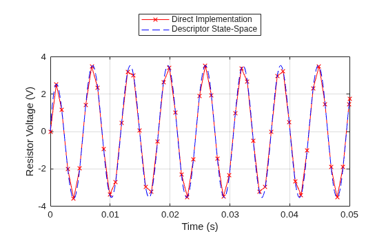
Both models produce the same simulation results. The implicit state-space model has a simpler block diagram and no algebraic loop.