Designing a High Angle of Attack Pitch Mode Control
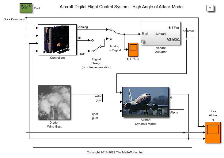
This example shows how to use Control System Toolbox™, Simulink® Control Design™ and Aerospace Blockset™ to design a flight control system for the longitudinal motion of aircraft. You develop a controller that enables stable operation at high angles of attack with minimal pilot workload.
Stick input from the pilot provides the reference angle of attack command. The controller uses pitch angle and pitch rate feedback to generate the elevator command, which is passed to the actuator subsystem. The actuator dynamics are implemented as a second-order system using actuator blocks from Aerospace Blockset, and the resulting actuator output is applied to the aircraft model. The aircraft dynamics are modeled using first-order linear approximations, and the model is perturbed with wind-gust disturbances generated using a simplified Dryden wind gust model.
Open the model. The Controllers and Actuator subsystems use variant configurations to switch between different control and actuator implementations.
open_system("slexAircraftPitchControlExample");
Trimming and Linearization
You can linearize the model interactively using the Model Linearizer (Simulink Control Design). On the Apps tab, under Control Systems, click Model Linearizer. You can also linearize programmatically with the linearize function.
Open the slexAircraftPitchControlAutopilot model.
apmdl = 'slexAircraftPitchControlAutopilot';
open_system(apmdl);
To view the linearized model parameters:
op = operpoint(apmdl);
io = getlinio(apmdl);
contap = linearize(apmdl,op,io)
contap =

  A =
                 Alpha-sensor  Pitch Rate L  Proportional  Stick Prefil
   Alpha-sensor        -2.526             0             0             0
   Pitch Rate L             0        -4.144             0             0
   Proportional         -1.71        0.9567             0            10
   Stick Prefil             0             0             0           -10

  B =
                 Alpha Sensed         Stick      q Sensed
   Alpha-sensor             1             0             0
   Pitch Rate L             0             0             1
   Proportional             0             0       -0.8156
   Stick Prefil             0             1             0

  C =
        Alpha-sensor  Pitch Rate L  Proportional  Stick Prefil
   Sum         2.986         -1.67        -3.864        -17.46

  D =
        Alpha Sensed         Stick      q Sensed
   Sum             0             0         1.424

Continuous-time state-space model.
Linear Time-Invariant (LTI) Systems
Linear time-Invariant (LTI) systems represent a linear model using state space (SS), transfer function (TF), or zero-pole-gain (ZPK) objects. The variable contap (CONTinuous AutoPilot) is a state-space object. Use this code to convert between object types as needed.
contap = tf(contap);
contap = zpk(contap);
To inspect LTI object properties, use the get command or access the properties directly, such as by using contap.InputName.
Discretized Controller Using Zero-Order Hold
Use the LTI object to design a discrete autopilot that matches the behavior of the analog design as closely as possible. For the initial design, use a zero-order hold (ZOH) with a sample time of 0.1 second to obtain a discrete version of the controller.
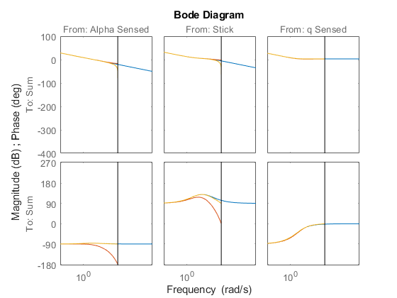
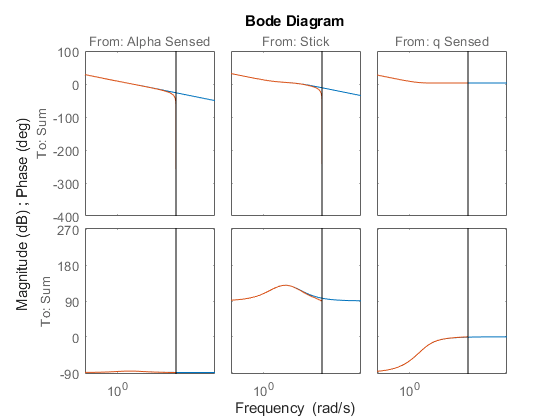
discap = c2d(contap, 0.1, 'zoh');
bode(contap,discap);
grid on;
legend('continuous','discreteZOH', 'Location', 'northeastoutside');
The Bode plot shows that the discrete and analog systems differ in phase from approximately 3 rad/sec to the half-sample frequency, indicating that the discrete design exhibits poorer phase characteristics than the analog system. When used in simulation, this discrete design can cause the closed-loop system to become unstable. To verify this behavior, simulate the model using the variant configurations. Right-click the Controllers subsystem, select the AnalogControl variant and then the LTI variants, and compare their corresponding responses.
Tustin (Bilinear) Discretization
To improve the performance, you can try different discretization methods. For example, try the Tustin transformation.
discap1 = c2d(contap,0.1,'tustin');
bode(contap,discap,discap1);
grid on;
legend('continuous','discreteZOH','discreteTustin', 'Location', 'northeastoutside');

Selecting a Sample Time
The Tustin method improves phase matching and performs better than the zero-order hold. However, the sample time of 0.1 second is too slow to track the performance of the analog system at half the sample frequency. You can verify this behavior by setting the object name in the LTI variant to discap1 and observing that the closed-loop system remains unstable.
To improve performance, decrease the sample time to 0.05 second.
discap = c2d(contap,0.05,'tustin');
bode(contap,discap);
grid on;
legend('continuous','discreteTustin', 'Location', 'northeastoutside');

The Bode plot confirms that the Tustin approximation with a sample time of 0.05 second better tracks the performance of the analog system. You can verify this behavior by running the simulation with the LTI variant. Check that the object name is set to discap before running the simulation.
With a workable discrete design in place, you can implement the controller with the additional practical elements that are not captured in the linear analysis.
Digital Implementation with Real-World Considerations
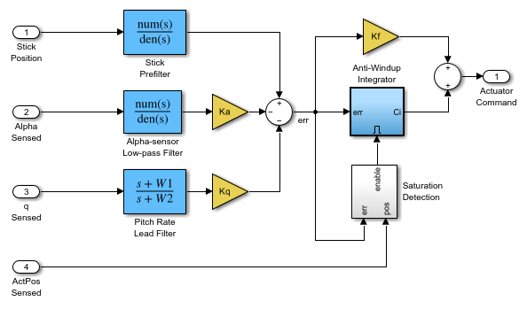
The analog controller provides a continuous-time design with prefilters, sensor dynamics, and an anti-windup integrator. While effective for analysis, you cannot implement this structure directly in an embedded system. To mitigate this limitation, consider digital implementation.
Open the AnalogControl variant.
open_system('slexAircraftPitchControlExample/Controllers/AnalogControl')
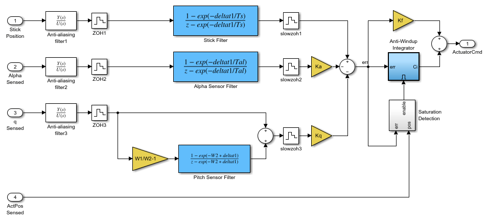
Implementing the controller digitally prevents high-frequency measurement noise from being aliased into the control bandwidth when signals are sampled. Once this aliasing occurs, the aliased components are indistinguishable from the true system dynamics. To avoid this issue, the digital implementation model inserts analog anti-aliasing filters ahead of the Zero-Order Hold blocks that model the analog-to-digital converters (ADCs). These filters limit the bandwidth of the measured signals, so only frequencies within the sampling bandwidth enter the digital controller.
In addition to the analog filters, the digital controller includes discrete filters that operate at a higher sampling rate than the main compensator. These filters condition the measured signals, providing improved noise rejection and more accurate inputs to the compensator. Their sample time, deltat1, is set to one-tenth of deltat, and the ZOH1, ZOH2, and ZOH3 blocks propagate these sample times to downstream components through sample-time inheritance.
The DigitalControl variant of the Controller subsystem implements these settings.
set_param('slexAircraftPitchControlExample/Controllers', 'LabelModeActiveChoice', 'DigitalControl')
set_param('slexAircraftPitchControlExample', 'SimulationCommand', 'update')
open_system('slexAircraftPitchControlExample/Controllers/DigitalControl')
You can increase the amplitude of the wind gust and verify that the anti-aliasing filters are working satisfactorily. To increase the gust amplitude, open the Dryden Wind Gust subsystem and change the noise variance of the White Noise block that drives the gust simulation.
Actuator Implementation
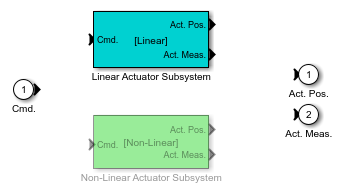
The Actuator subsystem uses variants to switch between linear and nonlinear implementations. The linear variant uses the Linear Second-Order Actuator (Aerospace Blockset) block. The nonlinear variant uses the Nonlinear Second-Order Actuator (Aerospace Blockset) block.
open_system('slexAircraftPitchControlExample/Actuator')
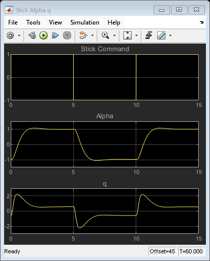
Aircraft Response at High Angle of Attack
You can examine the closed-loop response of the pitch controller at high angle of attack by simulating the model and plotting the stick command from the pilot and the resulting angle of attack. These results correspond to the DigitalControl variant.
out = sim('slexAircraftPitchControlExample');

figure(2);
plot(out.logsOut{1}.Values.Time, out.logsOut{1}.Values.Data); hold on;
plot(out.logsOut{2}.Values.Time, out.logsOut{2}.Values.Data);
grid on;
xlabel('Time (s)');
legend('alpha','stickCommand');
title('Time Response of the Aircraft Pitch Control');
Simulate the system again and switch among the three controller variant choices: AnalogControl, LTI, and DigitalControl. You should observe that the overall response is not significantly affected by which variant is active, confirming that the LTI and digital implementations preserve the behavior of the analog controller.
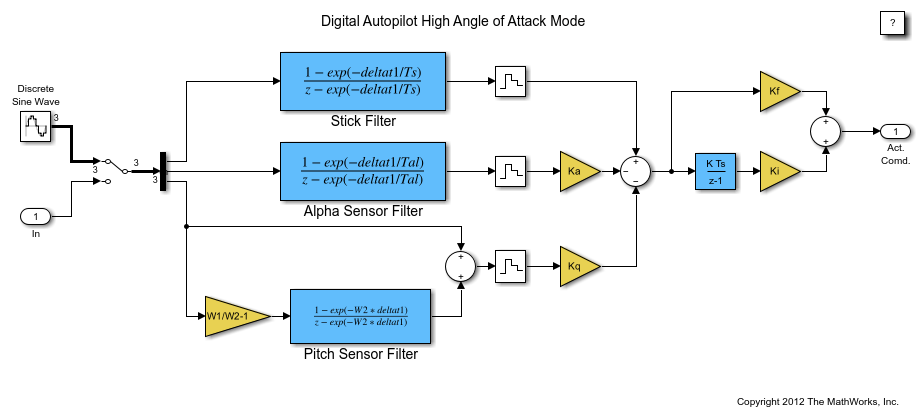
Code Generation
You can transform the digital autopilot into embeddable code using Simulink® Coder™.
open_system("slexAircraftPitchControlDAP")
Use the slbuild command to generate a standalone executable for the digital autopilot model slexAircraftPitchControlDAP. You can build and run the executable directly from MATLAB.
slbuild("slexAircraftPitchControlDAP")
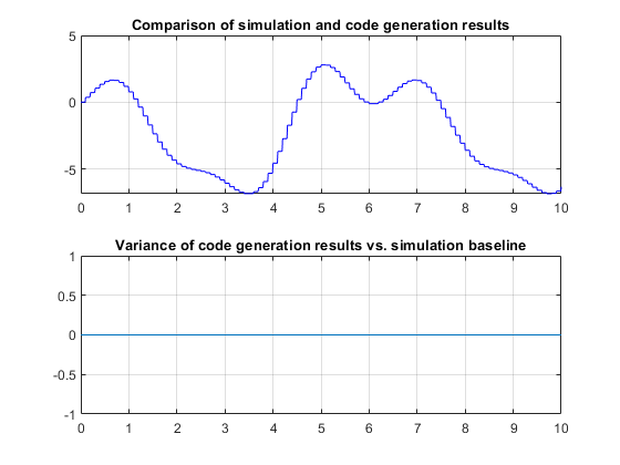
!slexAircraftPitchControlDAP.exeWhen executed, the program produces a MAT file, slexAircraftPitchControlDAP.mat, which contains the logged variables rt_tout and rt_yout. Load this file into the workspace to compare the generated-code output with the baseline Simulink® simulation.
load slexAircraftPitchControlDAP
For this model, the generated code results closely match the simulation output, with differences effectively zero on this host. In more complex designs, small numerical discrepancies can occur due to compiler optimizations, target-specific math libraries, or extended-precision intermediate register values. You should investigate larger differences, as they can indicate a numerical stability problem in the control algorithms or issues in the generated code.
sim("slexAircraftPitchControlDAP");

figure(3);
subplot(2,1,1);
plot(tout,yout,'r'); hold on;
plot(rt_tout,rt_yout,'b--');
grid on;
xlabel('Time (s)');
legend('Simulation Result','Generated-Code Result');
title('Comparison of Simulation and Code Generation Results');

yvar = rt_yout - yout;
subplot(2,1,2);
plot(tout,yvar); grid on;
xlabel('Time (s)');
title('Difference Between Simulation and Code Generation Results');
See Also
linearize (Simulink Control Design) | Model Linearizer (Simulink Control Design)
Topics
- Aerospace Blockset
- Create Aerospace Models (Aerospace Blockset)