Parameterize Entropic Coefficient with Measurement Protocol and Data Analysis

Since R2024a

This example shows what experiments to conduct and how to analyze the resulting experimental data for parameterizing the entropic coefficient. The entropic heat is a reversible heat generation term inside battery thermal models. This equation calculates the entropic heat,

${\dot{Q}}_{rev} = I * T * \frac{dU}{dT}$ ,

where I is the battery current, T is the battery temperature, and dU/dT is the entropic heat coefficient. The entropic heat coefficient mainly depends on the state of charge (SOC). The Battery Equivalent Circuit block provides the capability to model the reversible entropic heat by specifying the Reversible heat model and Entropic coefficient parameters.

To measure the entropic heat coefficient for a battery cell, you must sweep through different levels of SOCs and characterize the entropic heat coefficient one SOC at a time. To reach different SOC levels, first you feed pulsed discharge currents to the battery. Then you let the cells rest until they reach the electrochemical equilibrium. To shorten the required rest time for reaching the electrochemical equilibrium, the SOC sweeping discharge and rest are performed under a relatively higher environmental chamber temperature such as 30 degC.

These figure show the test used to characterize the entropic heat coefficient. The figure on the left shows the measured battery terminal voltage. The figure on the right shows the measured input current.

At each SOC, you thermally cycle the cell and measure the open-circuit voltage (OCV) at each temperature level after the cell temperature is close to the setpoint temperature of the environmental chamber. In these figures, the environmental chamber temperature setpoint cycles through 30, 40, 30, 20, 10, 5, 10, 20, and 30 degC consecutively.

To minimize the impact of voltage measurement noise from the battery tester and to calculate the entropic heat coefficient for the SOC, you perform a linear fit of the OCV over a range of temperature setpoints because the entropic heat coefficient is typically in the order of 0.1 mV/K, whereas the battery tester typically has a measurement accuracy of 1 mV.

Generate Synthetic Data

In real-world applications, you replace the Simscape model simulation with real experiments in a laboratory. The Simscape model in this example details the test procedure for the SOC and temperature sweep. You can then copy these details to the real-world experimental setup.

Open the ModelForSimulatingTest model.

open_system("ModelForSimulatingTest.slx")

This example already provides a properly-parameterized value for the OCV of the Battery Equivalent Circuit block to accurately reflect how the OCV changes with the temperature. To mimic the voltage measurement noise of the real world experiments, the model adds a band-limited white noise to the simulated voltage. This noise is set to 1mV standard deviation.

Simulate the model.

out=sim("ModelForSimulatingTest.slx");

Extract the time, voltage, SOC, temperature, and thermal equilibrium flag from the simulation data.

t = out.logsout{1}.Values.Time;
voltage = out.logsout{1}.Values.Data;
temperatureFlag = out.logsout{2}.Values.Data;
soc = out.logsout{4}.Values.Data;
T = out.logsout{3}.Values.Data;

Analyze Data for Calculation of Entropic Heat Coefficient

Use the synthetic data from the Simscape model to perform the analysis one SOC at a time by fitting the OCV data against temperature during thermal cycling.

To show the noisiness of the OCV data and the fitted OCV against the temperature line, this code plots the OCV over temperature at the SOC levels of 0, 0.5, and 1. If you have real-world experimental results available, you can replace the synthetic data.

dUdTExp = zeros(size(SOC_vec2));
figure(Position=[0 0 2000 600]);
tiledlayout(1,3)
for i = 1:numel(SOC_vec2)
    indx = find(abs(soc-SOC_vec2(i))<1.5e-3 & temperatureFlag == 1);
    dUdTfit = polyfit(T(indx), voltage(indx),1);
    T_x = linspace(min(T(indx)), max(T(indx)),100);
    dUdT_y = polyval(dUdTfit, T_x);
    if mod(i,10) == 1
        nexttile
        plot(T(indx), voltage(indx),'o', T_x, dUdT_y);
        xlabel('temperature (K)');
        ylabel('OCV (V)');
        title(sprintf('%.2f SOC',SOC_vec2(i)));
    end

    dUdTExp(1,i) = dUdTfit(1)*1000; % converting V/K to mV/K 
  
end

Notice that the voltage data is noisy, which is the case for real-world experimental data as well. However, the linear fit to obtain the slope of the fitted line addresses the noisy data issue. The slope of the fitted line, which represents the OCV against the temperature, can be positive or negative. This is expected because the entropic heat coefficient can be positive or negative. The sign for the entropic heat coefficient depends on the electrochemistry, stoichiometry, and SOC.

The entropic heat coefficient is then used to properly parameterize OCV for each SOC under different temperature in the Battery Equivalent Circuit block in the Simscape model.

Compare Measured Entropic Heat Coefficient Against Benchmark

Compare the results against the benchmark data used in the Simscape model for generating the synthetic data [1].

figure; plot(SOC_vec2, dUdTExp,'x', SOC_vec2,dUdT2, 's');
legend({'measured', 'benchmark'});
xlabel('SOC (-)');
ylabel('Entropic coefficient dU/dT (mV/K)')

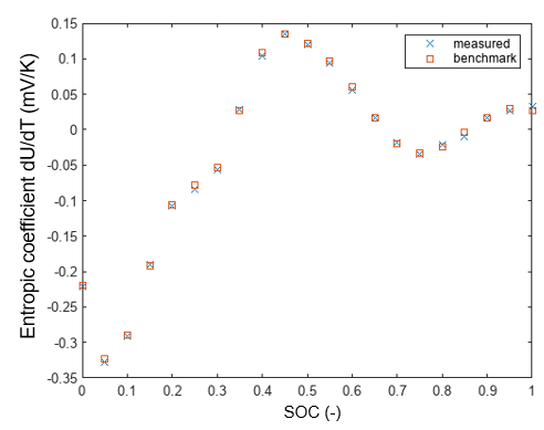
The measured entropic heat coefficient matches well with the benchmark values. The measurement procedure and data analysis approach work well in dealing with the voltage measurement noise issue in light of a very low magnitude of the entropic heat coefficient.

Implement Entropic Heat Coefficient in Battery Equivalent Circuit Block for Thermal Model

Load the parameterized entropic heat coefficient variable from the experimental measurement.

if ~exist('dUdTExp','var')
    load dUdTExp.mat;
end

Open the model.

open_system('ThermalModelWithEntropicHeat.slx');

Enable the reversible heat model of the Battery Equivalent Circuit block. Set the Reversible heat model parameter to EntropicCoefficient.

set_param('ThermalModelWithEntropicHeat/Battery Equivalent Circuit','ReversibleHeatModel','2');

Set the Entropic coefficient parameter to "dUdTExp".

set_param('ThermalModelWithEntropicHeat/Battery Equivalent Circuit', 'EntropicCoefficient', 'dUdTExp');

C_rate = [0.1 0.5 1 2];
figure(Position=[0 0 1600 400]);
tiledlayout(1,4)

for j = 1:numel(C_rate)
    
    set_param('ThermalModelWithEntropicHeat/PS Constant', 'constant', num2str(-C_rate(j)*27));
    set_param('ThermalModelWithEntropicHeat/Convective Heat Transfer', 'heat_tr_coeff', num2str(C_rate(j)^2*200));
    set_param('ThermalModelWithEntropicHeat','StopTime',num2str(3600/C_rate(j)));
    out = sim("ThermalModelwithEntropicHeat.slx");
    Q_entrop_ts = out.logsout{2}.Values;
    Q_resist_ts = out.logsout{1}.Values;
    TM_SOC_ts = out.logsout{5}.Values;


    nexttile
    plot(TM_SOC_ts.Data,Q_entrop_ts.Data,'--',TM_SOC_ts.Data,Q_resist_ts.Data*1000); 
    
    title(sprintf('Discharge rate %2.1f C', C_rate(j)))
    lgd=legend({'reversible heat','irreversible heat'}, Location="southwest");
    xlabel('SOC');
    ylabel('Heat generation rate (W)');
    ax = gca; ax.XDir = "reverse";
end
lgd.Layout.Tile = 'east';

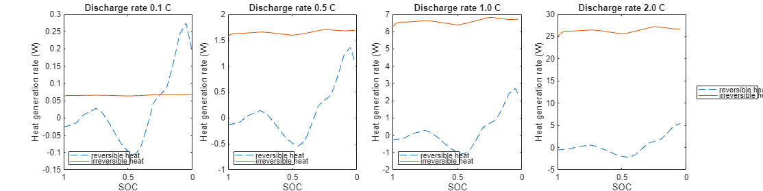
For the specific set of parameters in this example, the reversible heat is comparable to the irreversible heat for lower rate applications, such as those rates of 1C or lower. However, for higher C rates, the reversible heat starts to become negligible compared to the irreversible heat, which is expected because the majority of the irreversible heat comes from the resistive heat. The resistive heat is proportional to the current squared based on the Joule heating and Ohm's law. The entropic heat is proportional to the current, instead.

References

[1] Geng, Zeyang, et al. ‘A Time- and Cost-Effective Method for Entropic Coefficient Determination of a Large Commercial Battery Cell’. IEEE Transactions on Transportation Electrification, vol. 6, no. 1, Mar. 2020, pp. 257–66. DOI.org (Crossref), https://doi.org/10.1109/TTE.2020.2971454.