Simulate 5G NR FR2 MIMO Transmitter and Measure EVM
R2026bThis example shows how to generate a standard-compliant 5G New Radio (NR) Frequency Range 2 (FR2) 3GPP waveform, integrate the complete 8-chain MIMO transmitter into a MATLAB testbench using an RF system object, and measure the transmitter error vector magnitude (EVM).
Generate 5G NR FR2 Reference Waveform
To test the transmitter with a realistic signal, generate a standard-compliant 3GPP reference waveform. Use TM3.1 with 400 MHz bandwidth and 120 kHz subcarrier spacing in frequency division duplex (FDD) mode. These parameters represent a typical 5G FR2 deployment at 27 GHz.
rc = "NR-FR2-TM3.1";
bw = "400MHz";
scs = "120kHz";
dm = "FDD";
Set the sample rate to 491.52 MHz to satisfy the Nyquist criterion for the 400 MHz bandwidth signal.
Tstep = 1/491.52e6;
Tstop = 1.5e-4;
N = round(Tstop/Tstep);

tmwavegen = hNRReferenceWaveformGenerator(rc, bw, scs, dm);
tmwavegen = makeConfigWritable(tmwavegen);
tmwavegen.Config.SampleRate = 1/Tstep;
tmwavegen.Config.NumSubframes = 1;
[inWaveform, tmwaveinfo, resourcesinfo] = generateWaveform(tmwavegen,...
    tmwavegen.Config.NumSubframes);
inWaveform = inWaveform./max(abs(inWaveform)); % Normalize to unit peak for consistent power scaling
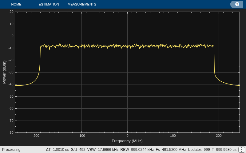
Visualize the spectrum of the 5G signal. Set the resolution bandwidth to 1 MHz to clearly resolve the signal bandwidth.
SpectAnalyzer = spectrumAnalyzer;
SpectAnalyzer.SampleRate = 1/Tstep;
SpectAnalyzer.ReferenceLoad = 1;
SpectAnalyzer.RBWSource = "Property";
SpectAnalyzer.RBW = 1e6;
SpectAnalyzer(inWaveform);
Measure Input Signal Power
To establish a baseline for comparison, measure the input signal power. The signal is an incident power wave, so use 1 Ohm reference impedance. Truncate to the simulation duration defined by Tstop.
inWaveform = inWaveform(1:N);
PowMet = powermeter(ReferenceLoad=1, WindowLength=length(inWaveform));
AvgPow = PowMet(inWaveform);
Compute the gain needed to set the input power to -30 dBm per chain plus 9 dB to compensate for the power divider loss (20*log10(8) ~ 9 dB).
G = -30+9-AvgPow(end);
InputPower = AvgPow(end)+G %#ok<NOPTS>
InputPower =

  -21.0000
Measure Baseline EVM
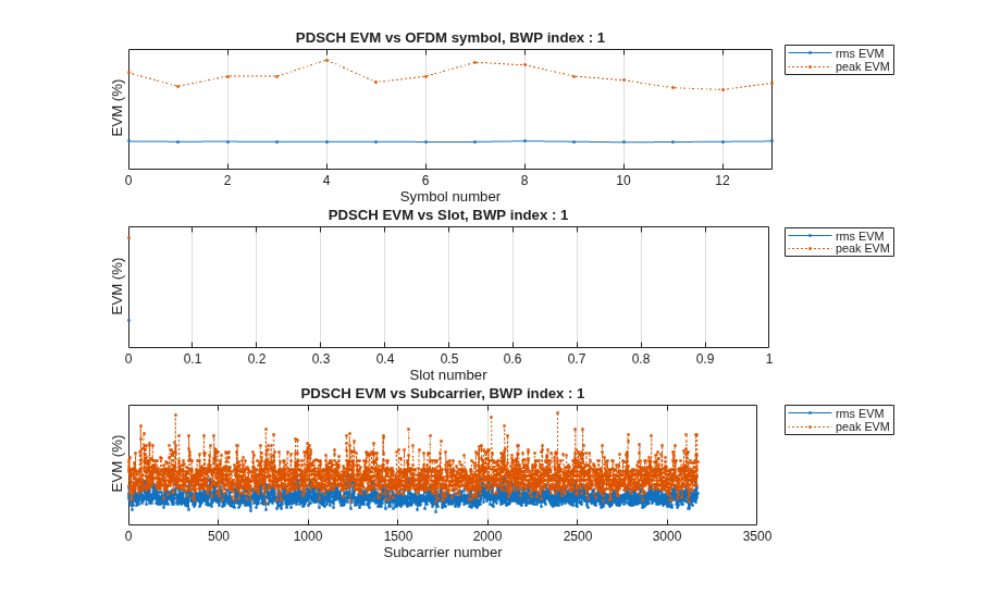
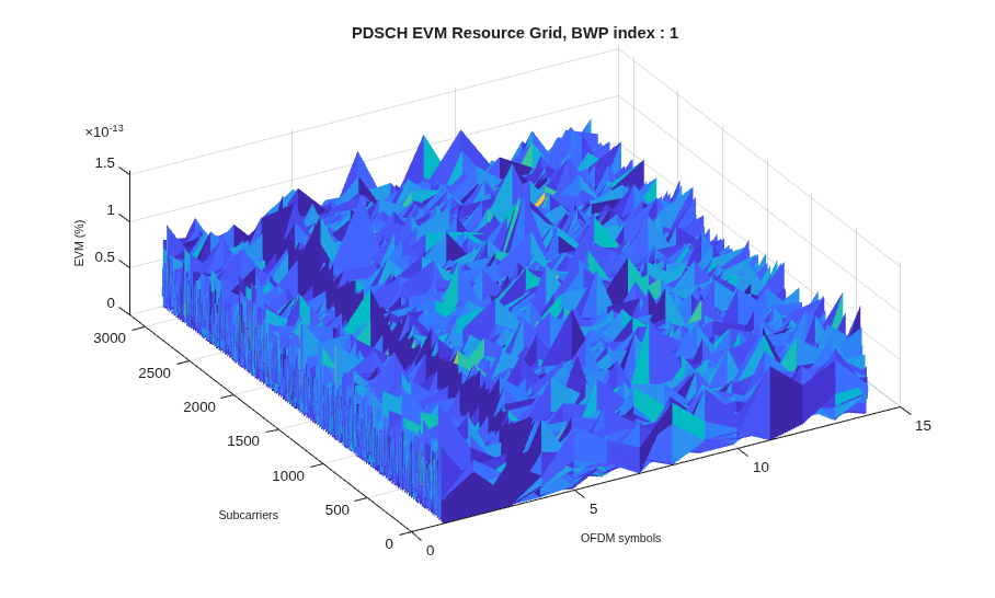
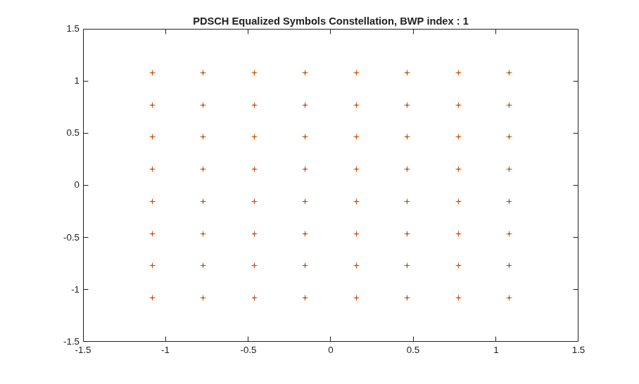
To establish the ideal EVM before RF impairments, configure the EVM measurement and compute it on the input waveform. The EVM measurement requires a reference baseband receiver with timing and phase recovery, channel equalization, and orthogonal frequency-division multiplexing (OFDM) demodulation.
cfg = struct();
cfg.Evm3GPP = false;
cfg.TargetRNTIs = [];
cfg.PlotEVM = true;
cfg.DisplayEVM = false;
cfg.Label = tmwavegen.ConfiguredModel{1};
cfg.UseWholeGrid = true;
cfg.PdcchEnable = false;

[evmInfo, ~, ~] = hNRDownlinkEVM(tmwavegen.Config, inWaveform, cfg);
BaselineEVM_RMS = evmInfo.PDSCH.OverallEVM.RMS*100 %#ok<NOPTS>
BaselineEVM_RMS =

   3.5490e-14
Integrate RF Transmitter into 5G Testbench
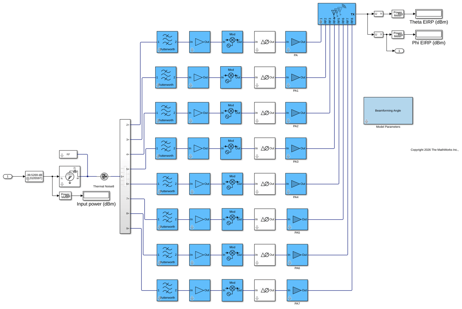
To simulate the complete transmitter chain in MATLAB, use an rfsystem System object. The rfsystem object wraps the Simulink model TX_8patch, which is derived from TXmodel_6 (Step 4) with these modifications to enable System object operation:
Added
In1/|Out1| ports (required byrfsystemfor the System object interface)Added a gain block to set the input drive level
Removed debug and monitoring blocks (per-chain outports, callback button)
Load the rfsystem object and the data it depends on. The underlying model requires these workspace variables:
patchArray- The 8-element antenna array object, used by the Antenna block for full-wave EM modeling.sSplitter- The power divider S-parameters (from Step 4), used by the corporate feed network block.
The model also uses phaseShifts and Az from its model workspace (configured in Step 3) and frequency variables (Fin, Flo, Fout) set by its own PreLoadFcn callback.
load("antennaData.mat");
load("splitterData.mat");
load("modelTX8.mat");
load("phaseShifterData.mat")
RF_TX.SampleTime = Tstep;
Open the Simulink model associated with the RF system object.
open_system(RF_TX);
Measure Transmitter Output Power and PAPR
The full transmitter simulation takes approximately 30 minutes. Load pre-computed results to measure output power and peak-to-average power ratio (PAPR).
% outWaveform = RF_TX(inWaveform.*db2mag(G));
% release(RF_TX);
% save("transmitterData.mat", "outWaveform");

load("transmitterData.mat");

PowMet = powermeter(ReferenceLoad=1, WindowLength=length(outWaveform),...
    Measurement="All");
[AvgPow, ~, PAPR] = PowMet(outWaveform);
OutputPower = AvgPow(end) %#ok<NOPTS>
OutputPAPR = PAPR(end) %#ok<NOPTS>
OutputPower =

   36.2085


OutputPAPR =

   10.7743
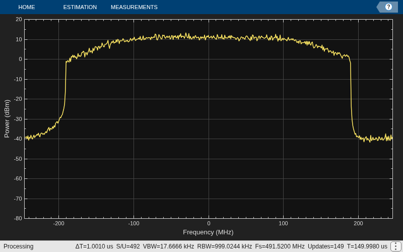
Measure the output spectrum to observe spectral regrowth from RF nonlinearities.
SpectAnalyzer = spectrumAnalyzer;
SpectAnalyzer.SampleRate = 1/Tstep;
SpectAnalyzer.ReferenceLoad = 1;
SpectAnalyzer.RBWSource = "Property";
SpectAnalyzer.RBW = 1e6;
SpectAnalyzer(outWaveform);
Measure Transmitter EVM
To quantify the signal distortion introduced by the RF chain, compute the EVM after passing through the complete transmitter. Compare this value to the baseline EVM measured earlier.
[evmInfo, ~, ~] = hNRDownlinkEVM(tmwavegen.Config, outWaveform, cfg);
TransmitterEVM_RMS = evmInfo.PDSCH.OverallEVM.RMS*100 %#ok<NOPTS>
TransmitterEVM_RMS =

    0.4015
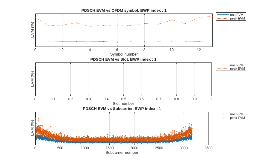
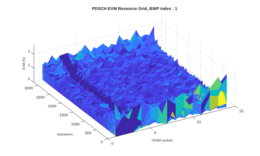
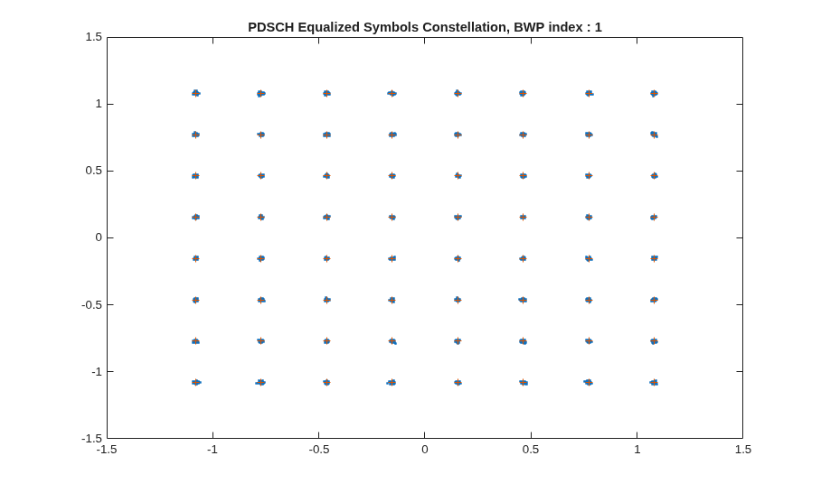
The RF transmitter chain increases EVM due to PA nonlinearity, phase noise, and filter distortion.
fprintf("Baseline EVM: %.2f%% -> Transmitter EVM: %.2f%%\n",...
    BaselineEVM_RMS, TransmitterEVM_RMS);
Baseline EVM: 0.00% -> Transmitter EVM: 0.40%

