Power Amplifier Characterization
This example shows how to characterize a power amplifier (PA) using measured input and output signals of an NXP Airfast PA. Optionally, you can use a hardware test setup including an NI PXI chassis with a vector signal transceiver (VST) to measure the signals at run time.
You can use the characterization results to simulate the PA using the comm.MemorylessNonlinearity (Communications Toolbox) System object™ or Memoryless Nonlinearity (Communications Toolbox) block. For a PA model with memory, you can use Power Amplifier block. You can use these models to design digital predistortion (DPD) using comm.DPD (Communications Toolbox) and comm.DPDCoefficientEstimator (Communications Toolbox) System objects or DPD (Communications Toolbox) and DPD Coefficient Estimator (Communications Toolbox) blocks. For more information, see Digital Predistortion to Compensate for Power Amplifier Nonlinearities (Communications Toolbox).
Optional Hardware and Software
This example can run on an NI PXI chassis with a VST to measure PA input and output signals during run time. The VST is a high-bandwidth RF instrument that combines a Vector Signal Generator (VSG) with a Vector Signal Analyzer (VSA). The following NI PXI chassis configuration was used to capture the saved signal:
NI PXIe-5840 Vector Signal Transceiver (VST)
NI PXIe-4139 Source Measure Unit (SMU)
NI PXIe-4145 SMU
NI RFmx SpecAn software
NI-RFSG software
NI-RFSG Playback Library software
As the device under test (DUT), this example uses an NXP Airfast LDMOS Doherty PA with operating frequency 3.6-3.8 GHz and 29 dB gain. This PA requires 29V, 5V, 3 V, 1.6V and 1.4V DC bias, which are provided using PXIe-4139 and PXIe-4145 SMUs.
Install MATLAB® on the NI PXI controller to run this example with the hardware setup, which is illustrated in the following figure. MATLAB, running on the PXI controller, generates test waveform and downloads the waveform to the VSG. The VSG transmits this test waveform to the PA and the VSA receives the impaired waveform at the PA output. MATLAB collects the PA output from the VSA and performs PA characterization.

Set dataSource variable to "Hardware" to run a test signal though the PA using the hardware setup described above. The test signal can be either a 5G-like OFDM waveform or two tones, as described in the following section. Set dataSource variable to "From file" to use prerecorded data.
dataSource =  "From file";
Generate Test Signals
To generate a test signal, specify the type of test signal as "OFDM" or "Tones". Specifying the testSignal as "OFDM" uses a 5G-like OFDM waveform with 64-QAM modulated signals for each subcarrier. "Tones" uses two tones at 1.8 MHz and 2.6 MHz, to test the intermodulation caused by the PA.
The example will use an oversampling factor of 7 to run the grid search up to an expected seventh-order nonlinearity, and normalize the waveform amplitude.
testSignal ="OFDM"; switch testSignal case "OFDM" bw =
100e6; [txWaveform,sampleRate,numFrames] = helperPACharGenerateOFDM(bw); case "Tones" bw = 3e6; [txWaveform,sampleRate,numFrames] = helperPACharGenerateTones(); end txWaveform = txWaveform/max(abs(txWaveform)); % Normalize the waveform
Hardware Test
If the dataSource variable is set to "From file", load the prerecorded data. If the dataSource variable is set to "Hardware", run the test signal through the PA using the VST. Create a helperVSTDriver object to communicate with the VST device. Set the resource name to the resource name assigned to the VST device. This example uses 'VST_01'. For NI devices, you can find the resource name using the NI Measurement & Automation Explorer (MAX) application.
if strcmp(dataSource, "Hardware")
  VST = helperVSTDriver('VST_01');
Set the expected gain values of the DUT and the attenuator. Since PA output is connected to a 30 dB attenuator, set VSA external attenuation to 30. Set the expected gain of the DUT to 29 dB and gain accuracy to 1 dB. Set the acquisition time to a value that will result in about 40k samples. Set the target input power to 8 dBm. You can increase this value to drive the PA more into the non-linear region.
  VST.DUTExpectedGain     = 29;     % dB
  VST.ExternalAttenuation = 30;     % dB
  VST.AcquisitionTime     = 0.9e-3*(53.76e6/sampleRate); % seconds
  VST.DUTTargetInputPower =8;  % dBm
  VST.CenterFrequency     = 3.7e9   % Hz
Download the test waveform to the VSG. Measure PA output.
  writeWaveform(VST,txWaveform,sampleRate,testSignal)
  results = runPAMeasurements(VST);
  release(VST)
else
  % Load the prerecorded results from VST
  switch testSignal
    case "OFDM"
      dataFileName = sprintf("helperPACharSavedData%dMHz",bw/1e6);
    case "Tones"
      dataFileName = "helperPACharSavedDataTones";
  end
  load(dataFileName,"results","sampleRate","overSamplingRate","testSignal","numFrames")
end
Map results into local variables.
referencePower = results.ReferencePower;
measuredAMToAM = results.MeasuredAMToAM;
paInput = results.InputWaveform;
paOutput = results.OutputWaveform;
linearGaindB = results.LinearGain;
Plot the spectrum of the test signal using the spectrumAnalyzer (DSP System Toolbox) function.
saInput = helperPACharPlotInput(paInput, sampleRate, testSignal, bw);

Plot the AM/AM characteristics of the PA.
helperPACharPlotSpecAnAMAM(referencePower, measuredAMToAM)

For a better view, focus on gain vs input power instead of output power vs input power and plot again.
helperPACharPlotSpecAnGain(referencePower, measuredAMToAM)

The PA is mostly linear of the input power range -1 to 17 dBm, with only about 1dB variation over that range. The width of the gain curve is due to the memory effects of the PA.
PA Characterization
Use the measured PA input and output data to model the PA. Then, you can use this model to simulate a system that contains this PA and fine tune the parameters. This example considers three models: memoryless nonlinearity, memory polynomial and memory polynomial with cross terms.
Memoryless Nonlinearity Model
Memoryless nonlinear impairments distort the input signal amplitude and phase. The amplitude distortion is amplitude-to-amplitude modulation (AM/AM) and the phase distortion is amplitude-to-phase modulation (AM/PM). The comm.MemorylessNonlinearity (Communications Toolbox) System object and Memoryless Nonlinearity (Communications Toolbox) block implements several such distortions. Use the PA input and output data to create a lookup table to use with this object or block.
To characterize the AM/AM transfer function, calculate the average output power for a range of input power values. Measurements are in volts over an overall 100 ohm impedance, split between the transmitter and receiver. Convert the measured baseband samples to power values in dBm. The +30 dB term is for dBW to dBm conversion and the -20 dB term is for the 100 ohm impedance.
paInputdBm  = mag2db(abs(paInput)) + 30 - 20;
paOutputdBm  = mag2db(abs(paOutput)) + 30 - 20;
Partition the input power values into bins. The edges variable contains the bin edges, and the idx variable contains the index of the bin values for each input power value.
[N,edges,idx] = histcounts(paInputdBm, 'BinWidth', 0.5);For each bin, calculate the midpoint of the bin, average output power and average phase shift. Do not include any input power value that is less than 20 dB below the maximum input power. Store the results in a three-column matrix where the first column is the input power in dBm, second column is the output power in dBm and last column is the phase shift.
minInPowerdBm = max(paInputdBm) - 20;
minIdx = find(edges < minInPowerdBm, 1, 'last');
tableLen = length(edges)-minIdx-1;
inOutTable = zeros(tableLen,2);
for p = minIdx+1:length(edges)-1
  inOutTable(p-minIdx,1) = mean(paInputdBm(idx == p));   % Average input power for current bin
  inOutTable(p-minIdx,2) = mean(paOutputdBm(idx == p));  % Average output power for current bin
  inOutTable(p-minIdx,3) = mean(angle(paOutput(idx == p)./paInput(idx == p)));  % Average phase shift for current bin
end
Use the table in the comm.MemorylessNonlinearity System object to model the PA. Compare the estimated output with the actual output.
pa = comm.MemorylessNonlinearity('Method','Lookup table','Table',inOutTable,'ReferenceImpedance',100)
pa =
  comm.MemorylessNonlinearity with properties:

                Method: 'Lookup table'
                 Table: [40×3 double]
    ReferenceImpedance: 100
paOutputFitMemless = pa(paInput);
err = paOutput - paOutputFitMemless;
rmsErrorMemless = rms(err)/rms(paOutput)*100;
disp(['Percent RMS error in time domain is ' num2str(rmsErrorMemless) '%'])
Percent RMS error in time domain is 6.562%
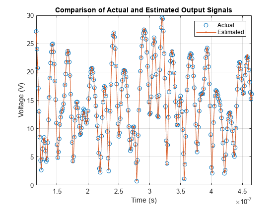
To visualize both the measured output signal and the fitted output signal, plot the actual and fitted time-domain output voltages.
helperPACharPlotTime(paOutput, paOutputFitMemless, sampleRate)

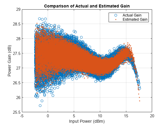
Plot the magnitude of the gain.
helperPACharPlotGain(paInput, paOutput, paOutputFitMemless)

Memory Polynomial Model
The memory polynomial model includes the memory effects of the PA in addition to the nonlinear gain. Use the multipurpose helper function helperPACharMemPolyModel to determine the complex coefficients of a memory polynomial model for the amplifier characteristics. Set the model type to 'Memory Polynomial'.
modType =  'memPoly';
Perform a grid search as shown in Appendix Grid Search for Memory Length and Polynomial Order. Based on this grid search results, the best fit is obtained when memory length and polynomial degree values are as follows:
memLen = 5;
degLen = 5;
Perform the fit and RMS error calculation for these values. Only half of the data is used to compute the fitting coefficients, as the whole data set will be used to compute the relative error. The helper function helperPACharMemPolyModel calculates the coefficients of the model.
numDataPts = length(paInput);
halfDataPts = round(numDataPts/2);
The helper function helperPACharMemPolyModel is editable for custom modifications, and to return the desired matrix. The PA model has some zero valued coefficients, which results in a rank deficient matrix.
fitCoefMatMem = helperPACharMemPolyModel('coefficientFinder',             ...
  paInput(1:halfDataPts),paOutput(1:halfDataPts),memLen,degLen,modType);
Warning: Rank deficient, rank = 24, tol = 1.870608e-01.
disp(abs(fitCoefMatMem))
   23.1550    8.8545   17.8391   13.3029    3.2169
         0   11.7683   26.4688   23.1943    5.5478
   20.9756   16.8535   25.7350   22.1938    5.0691
   32.6215    8.4047    9.4917   10.6995    2.5616
   15.3881    2.3632    2.0872    2.9343    0.7371
To validate the fitting, use the helper function to compute percent RMS error with respect to the measured signal.
rmsErrorTimeMem = helperPACharMemPolyModel('errorMeasure', ...
  paInput, paOutput, fitCoefMatMem, modType);
disp(['Percent RMS error in time domain is ' num2str(rmsErrorTimeMem) '%'])
Percent RMS error in time domain is 2.5023%
To visualize both the measured output signal and the fitted output signal, plot the actual and fitted time-domain output voltages.
paOutputFitMem = helperPACharMemPolyModel('signalGenerator', ...
  paInput, fitCoefMatMem, modType);
helperPACharPlotTime(paOutput, paOutputFitMem, sampleRate)

Plot the magnitude of the gain.
helperPACharPlotGain(paInput, paOutput, paOutputFitMem)

Discussions
The percent RMS estimation error in time domain for the memoryless nonlinearity model, which is around 6%, is about 3 times more than the error for the memory polynomial model is, which is around 2%, for the OFDM signals with different bandwidths.
Check the estimation error in frequency domain by plotting the spectrum of the actual PA output together with the spectrum of the estimated PA output for all three models. The memoryless nonlinearity table lookup model is not able to simulate the spectral growth seen in the measured PA output. For this PA, memory polynomial model provides a good approximation of the PA characteristics.
sa = helperPACharPlotSpectrum(...
  [paOutput paOutputFitMemless paOutputFitMem],...
  {'Actual PA Output','Memoryless Model Output', ...
  'Memory Polynomial Output'},...
  sampleRate,testSignal);


The helper function helperPACharMemPolyModel can also use the memory polynomial with cross terms model, which includes the leading and lagging memory cross terms in addition to the memory effects of the PA and the nonlinear gain. Set the model type to 'Cross-Term Memory' to explore this model.
For further exploration, try different memory length and polynomial degree combinations. Modify the oversampling factor and explore its effect on the PA model performance. Modify the helper function helperPACharMemPolyModel to try different PA models.
Using PA Model for DPD Testing
Save the coefficient matrix of the PA model to be used in the Power Amplifier block for simulation at the system-level in the Digital Predistortion to Compensate for Power Amplifier Nonlinearities (Communications Toolbox).
frameSize = floor(length(paInput)/numFrames);
paIn.signals.values = double(reshape(paInput(1:frameSize*numFrames,1),numFrames,frameSize));
paIn.signals.dimensions = frameSize;
paIn.time = [];
save('PAcoefficientsAndInput.mat','modType','fitCoefMatMem','memLen','degLen','paIn','linearGaindB')
Appendix: Grid Search for Memory Length and Polynomial Order
Uncomment following lines to perform the grid search when the cost function is the percent RMS error in time. First choose the model type.
modType ='memPoly'; % rmsErrorTime = helperPACharGridSearchTime(paInput,paOutput,modType,overSamplingRate)
Repeat the search when the cost function is the percent RMS error in frequency.
% rmsErrorFreq = helperPACharGridSearchFrequency(paInput,paOutput,modType,overSamplingRate)