RF PCB
Libraries:
RF Blockset /
Circuit Envelope /
PCB
Description
The RF PCB block enables you to create, visualize, and analyze the characteristics of the
components used on a printed circuit board (PCB) in RF Blockset™ circuit envelope simulation environment. You can create components like
transmission lines, splitters, couplers, baluns, and many more from the PCB Components Catalog (RF PCB Toolbox) except the
viaSingleEnded object.
Note
To use this block, you need a RF PCB Toolbox™ license.
Examples
This example compares the coupler created using the S-parameter Coupler block and the RF PCB block. There are several types of coupler configurations an RF system can use, including quadrature, split-ring, and rat-race. This example compares the rat-race couplers created using the S-parameter Coupler block and the RF PCB block.
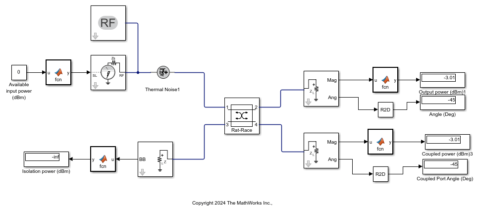
Rat-Race Coupler Using S-Parameter Coupler Block
The Coupler block models a four-port rat-race coupler in a circuit envelope environment as an ideal S-parameter model. This device consists of four ports: an input port, a through port, an isolated port, and a coupling port. The rat-race coupler designed using the Coupler block has a loss and coupling of around 3 dB, with the isolation being infinite. Additionally, the phase differences between the ports are equal.
Simulate this model and observe the results at the output, coupling, and isolation ports. The isolation of this coupler is infinite, and the output and phase difference at the output and coupling ports are the same.
open_system("IdealRateRace.slx") sim("IdealRateRace.slx")
ans =
Simulink.SimulationOutput:
tout: [1x1 double]
SimulationMetadata: [1x1 Simulink.SimulationMetadata]
ErrorMessage: [0x0 char]

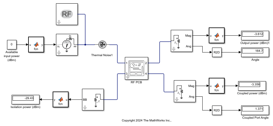
Rat-Race Coupler Using RF PCB Block
Use the RF PCB block to create a rat-race coupler from a object created using RF PCB Toolbox™.couplerRatrace (RF PCB Toolbox)
cr = couplerRatrace; sparam = sparameters(cr,linspace(1e9,5e9,16));
The RF PCB block enables you to create, visualize, and analyze the characteristics of the components used on a PCB in RF Blockset™ circuit envelope simulation environment. You can create components like transmission lines, splitters, couplers, baluns, and many more from the PCB component catalog from RF PCB Toolbox.
Simulate this rat-race model designed using the RF PCB block and observe the results at the output, coupling, and isolation ports. The rat-race coupler object is solved using the Method of Moments (MoM) solver. This coupler also has four ports: an input port, a through port, an isolated port, and a coupling port. However, in this design, the loss and coupling can vary depending on the design, and the isolation is approximately 29 dB. The phase difference between the through port and the coupling port is 180 degrees.
open_system("RFPCBRateRace.slx") sim("RFPCBRateRace.slx")
ans =
Simulink.SimulationOutput:
tout: [1x1 double]
SimulationMetadata: [1x1 Simulink.SimulationMetadata]
ErrorMessage: [0x0 char]

The rat-race coupler designed using the Coupler block allows you to model an ideal frequency-independent coupler with S-parameters, whereas the rat-race coupler designed using the RF PCB block allows you to design a coupler by specifying its physical properties, such as width and length, and enables you to simulate using MoM.
Parameters
To edit block parameters interactively, use the Property Inspector. From the Simulink® Toolstrip, on the Simulation tab, in the Prepare gallery, select Property Inspector.
Main
RF PCB Toolbox objects from the workspace. You can input any one of the objects from
the PCB Components Catalog (RF PCB Toolbox) except the
viaSingleEnded object.
Note
Analyze the RF PCB objects in the workspace for at least one frequency before using them in the block.
For example, to analyze an RF PCB object, you can input the RF PCB object to an
sparameters(RF PCB Toolbox) object.
RF PCB Geometry
Select this button to visualize all the metal layers and the PCB shape of the RF PCB component in the figure window. The red filled circle correspond to PCB feed points and the blue filled circles correspond to vias.
Dependencies
To visualize the layout, first input a PCB object from your workspace Object parameter and then select Apply button. Finally, select the Layout button.
Select this button to visualize the 3-D geometry of the RF PCB component in the figure window.
Dependencies
To visualize the layout, first input a PCB object from your workspace Object parameter and then select Apply button. Finally, select the 3D Geometry button.
Noise and RF Terminals
Select this parameter to simulate thermal noise in the antenna due to the real part of the impedance see at the antenna terminals.
Dependencies
To simulate thermal noise in this block, first select Simulate noise in the Configuration block.
Select this option to ground and hide the negative terminals. Clear this parameter to expose the negative terminals. By exposing these terminals, you can connect them to other parts of your model.
Modeling
To enable this tab, analyze the RF PCB objects in the workspace for at least one frequency.
Model S-parameters, specified as:
Time domain— This option creates an analytical rational model that approximates the whole range of the data.Frequency domain— This option computes the baseband impulse response for each carrier frequency independently. This technique is based on convolution. For more information, see Compare Time and Frequency Domain Simulation Options for S-parameters.
Time Domain Modeling
Data fitting options, specified as Fit individually,
Share poles by column, or Share all
poles. This parameter enables you to fit your data using
rational object.
The results of the fitted data is displayed under Rational fitting results section. The block displays Number of independent fits, Number of required poles, and Relative error achieved (dB).
Dependencies
To set this parameter, select Time domain in
Modeling options.
Relative error acceptable for the rational fit, specified as a scalar in decibels.
Dependencies
To set this parameter, select Time domain in
Modeling options.
Frequency Domain Modeling
Select this parameter to automatically calculate impulse response. Clear this parameter to manually specify the impulse response duration using Impulse response duration.
Dependencies
To set this parameter, select Frequency domain in
Modeling options.
Impulse response duration, specified as a scalar in seconds.
Dependencies
To set this parameter, first select Frequency domain
in Modeling options. Then, clear Automatically
estimate impulse response duration.
Visualization
To enable this tab, analyze the RF PCB objects in the workspace for at least one frequency.
Frequency data source, specified as:
When Source of frequency data is Extracted from
data source, the Data source must be set to
Data file. Verify that the specified Data
file contains frequency data.
When Source of frequency data is
User-specified, specify a vector of frequencies in the
Frequency data parameter. Also, specify units from the
corresponding drop-down list.
Frequency data range, specified as a finite vector.
Dependencies
To enable this parameter, set Source of frequency data to
User-specified.
Type of data plot that you want to produce with your data specified as one of the following:
X-Y plane— Generate a Cartesian plot of your data versus frequency. To create linear, semilog, or log-log plots, set the Y-axis scale and X-axis scale accordingly.Polar plane— Generate a polar plot of your data. The block plots only the range of data corresponding to the specified frequencies.Z smith chart,Y smith chart, andZY smith chart— Generate a Smith® chart. The block plots only the range of data corresponding to the specified frequencies.
Type of S-Parameters to plot, specified as S(1,1),
S(1,2), S21, or S22.
Type of S-Parameters to plot, specified as S(1,1),
S(1,2), S(2,1), or S(2,2).
Plot format, specified as Magnitude (dB),
Angle(degrees), Real, or
Imaginary.
Dependencies
To enable this parameter, set Plot type to X-Y
plane.
Plot format, specified as Magnitude (dB),
Angle(degrees), Real, or
Imaginary.
Dependencies
To enable this parameter, set Plot type to X-Y
plane.
Y-axis scale, specified as Linear or
Logarithmic.
Dependencies
To enable this parameter, set Plot type to X-Y
plane.
X-axis scale, specified as Linear or
Logarithmic.
Dependencies
To enable this parameter, set Plot type to X-Y
plane.
Select this button to plot the specified data.
Version History
Introduced in R2025a
MATLAB Command
You clicked a link that corresponds to this MATLAB command:
Run the command by entering it in the MATLAB Command Window. Web browsers do not support MATLAB commands.
Select a Web Site
Choose a web site to get translated content where available and see local events and offers. Based on your location, we recommend that you select: .
You can also select a web site from the following list
How to Get Best Site Performance
Select the China site (in Chinese or English) for best site performance. Other MathWorks country sites are not optimized for visits from your location.
Americas
- América Latina (Español)
- Canada (English)
- United States (English)
Europe
- Belgium (English)
- Denmark (English)
- Deutschland (Deutsch)
- España (Español)
- Finland (English)
- France (Français)
- Ireland (English)
- Italia (Italiano)
- Luxembourg (English)
- Netherlands (English)
- Norway (English)
- Österreich (Deutsch)
- Portugal (English)
- Sweden (English)
- Switzerland
- United Kingdom (English)