bar
Plot magnitudes of means and standard deviations of elementary effects
Since R2021b
Description
h = bar(eeObj)h. The color shading of each bar represents a histogram
representing values at different times. Darker colors mean that those values occur more
often over the whole time course. The plot shows a single dot for scalar or constant model
responses instead of a bar.
h = bar(eeObj,Name=Value)
Examples
Load the tumor growth model.
sbioloadproject tumor_growth_vpop_sa.sbprojGet a variant with estimated parameters and the dose to apply to the model.
v = getvariant(m1);
d = getdose(m1,'interval_dose');
Get the active configset and set the tumor weight as the response.
cs = getconfigset(m1);
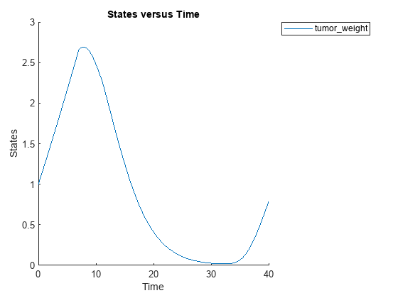
cs.RuntimeOptions.StatesToLog = 'tumor_weight';Simulate the model and plot the tumor growth profile.
sbioplot(sbiosimulate(m1,cs,v,d));
Perform global sensitivity analysis (GSA) on the model to find the model parameters that the tumor growth is sensitive to.
First, define model parameters of interest, which are involved in the pharmacodynamics of the tumor growth. Define the model response as the tumor weight.
modelParamNames = {'L0','L1','w0','k1'};
outputName = 'tumor_weight';
Then perform GSA by computing the elementary effects using sbioelementaryeffects. Use 100 as the number of samples and set ShowWaitBar to true to show the simulation progress.
rng('default');
eeResults = sbioelementaryeffects(m1,modelParamNames,outputName,Variants=v,Doses=d,NumberSamples=100,ShowWaitbar=true);
Show the median model response, the simulation results, and a shaded region covering 90% of the simulation results.
plotData(eeResults,ShowMedian=true,ShowMean=false);
![Figure contains an axes object. The axes object with xlabel time, ylabel [Tumor Growth].tumor indexOf w baseline eight contains 12 objects of type line, patch. These objects represent model simulation, 90.0% region, median value.](../../examples/simbio/win64/PerformGSAByComputingElementaryEffectsExample_02.png)
You can adjust the quantile region to a different percentage by specifying Alphas for the lower and upper quantiles of all model responses. For instance, an alpha value of 0.1 plots a shaded region between the 100*alpha and 100*(1-alpha) quantiles of all simulated model responses.
plotData(eeResults,Alphas=0.1,ShowMedian=true,ShowMean=false);
![Figure contains an axes object. The axes object with xlabel time, ylabel [Tumor Growth].tumor indexOf w baseline eight contains 12 objects of type line, patch. These objects represent model simulation, 80.0% region, median value.](../../examples/simbio/win64/PerformGSAByComputingElementaryEffectsExample_03.png)
Plot the time course of the means and standard deviations of the elementary effects.
h = plot(eeResults);
% Resize the figure.
h.Position(:) = [100 100 1280 800];![Figure contains 8 axes objects. Axes object 1 with xlabel time, ylabel std. of effects k1 contains an object of type line. Axes object 2 with xlabel time, ylabel mean of effects k1 contains an object of type line. Axes object 3 with ylabel std. of effects w0 contains an object of type line. Axes object 4 with ylabel mean of effects w0 contains an object of type line. Axes object 5 with ylabel std. of effects L1 contains an object of type line. Axes object 6 with ylabel mean of effects L1 contains an object of type line. Axes object 7 with title sensitivity output [Tumor Growth].tumor_weight, ylabel std. of effects L0 contains an object of type line. Axes object 8 with title sensitivity output [Tumor Growth].tumor_weight, ylabel mean of effects L0 contains an object of type line.](../../examples/simbio/win64/PerformGSAByComputingElementaryEffectsExample_04.png)
The mean of effects explains whether variations in input parameter values have any effect on the tumor weight response. The standard deviation of effects explains whether the sensitivity change is dependent on the location in the parameter domain.
From the mean of effects plots, parameters L1 and w0 seem to be the most sensitive parameters to the tumor weight before the dose is applied at t = 7. But, after the dose is applied, k1 and L0 become more sensitive parameters and contribute most to the after-dosing stage of the tumor weight. The plots of standard deviation of effects show more deviations for the larger parameter values in the later stage (t > 35) than for the before-dose stage of the tumor growth.
You can also display the magnitudes of the sensitivities in a bar plot. Each color shading represents a histogram representing values at different times. Darker colors mean that those values occur more often over the whole time course.
bar(eeResults);
![Figure contains an axes object. The axes object with title sensitivity output [Tumor Growth].tumor_weight, xlabel elementary effects, ylabel sensitivity input contains 18 objects of type patch, line. These objects represent mean, standard deviation.](../../examples/simbio/win64/PerformGSAByComputingElementaryEffectsExample_05.png)
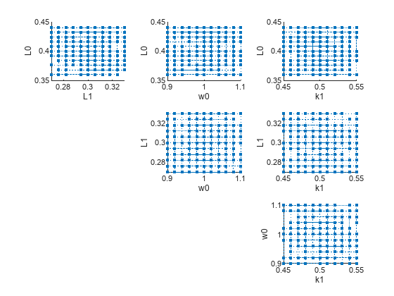
You can also plot the parameter grids and samples used to compute the elementary effects.
plotGrid(eeResults)
You can specify more samples to increase the accuracy of the elementary effects, but the simulation can take longer to finish. Use addsamples to add more samples.
eeResults2 = addsamples(eeResults,200);
The SimulationInfo property of the result object contains various information for computing the elementary effects. For instance, the model simulation data (SimData) for each simulation using a set of parameter samples is stored in the SimData field of the property. This field is an array of SimData objects.
eeResults2.SimulationInfo.SimData
   SimBiology SimData Array : 1500-by-1

   Index:    Name:         ModelName:         DataCount:
   1           -           Tumor Growth Model 1
   2           -           Tumor Growth Model 1
   3           -           Tumor Growth Model 1
   ...
   1500        -           Tumor Growth Model 1
You can find out if any model simulation failed during the computation by checking the ValidSample field of SimulationInfo. In this example, the field shows no failed simulation runs.
all(eeResults2.SimulationInfo.ValidSample)
ans = logical
   1
You can add custom expressions as observables and compute the elementary effects of the added observables. For example, you can compute the effects for the maximum tumor weight by defining a custom expression as follows.
% Suppress an information warning that is issued.
warnSettings = warning('off', 'SimBiology:sbservices:SB_DIMANALYSISNOTDONE_MATLABFCN_UCON');
% Add the observable expression.
eeObs = addobservable(eeResults2,'Maximum tumor_weight','max(tumor_weight)','Units','gram');
Plot the computed simulation results showing the 90% quantile region.
h2 = plotData(eeObs,ShowMedian=true,ShowMean=false);
h2.Position(:) = [100 100 1500 800];
![Figure contains 2 axes objects. Axes object 1 with ylabel Maximum tumor_weight contains 12 objects of type line, patch. One or more of the lines displays its values using only markers These objects represent model simulation, 90.0% region, median value. Axes object 2 with xlabel time, ylabel [Tumor Growth].tumor_weight contains 12 objects of type line, patch. These objects represent model simulation, 90.0% region, median value.](../../examples/simbio/win64/PerformGSAByComputingElementaryEffectsExample_07.png)
You can also remove the observable by specifying its name.
eeNoObs = removeobservable(eeObs,'Maximum tumor_weight');Restore the warning settings.
warning(warnSettings);
Input Arguments
Name-Value Arguments
Output Arguments
Version History
Introduced in R2021b