predict
Simulate and evaluate fitted SimBiology model
Syntax
Description
[
returns simulation results ynew,parameterEstimates]
= predict(resultsObj)ynew from evaluating the fitted SimBiology® model. The estimated parameter values parameterEstimates
used to compute ynew are from the original fit by
sbiofitmixed.
[
returns simulation results ynew,parameterEstimates]
= predict(resultsObj,data,dosing)ynew from evaluating the fitted SimBiology model by using the specified data and
dosing information.
[
uses additional options specified by one or more name-value arguments.ynew,parameterEstimates]
= predict(___,Name,Value)
Tip
Use this method to get model responses at specific time points or to predict model responses using different covariate data and dosing information.
Examples
Estimate nonlinear mixed-effects parameters using clinical pharmacokinetic data collected from 59 infants. Evaluate the fitted model given new data or dosing information.
Load Data
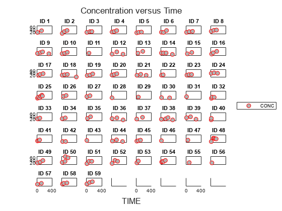
This example uses data collected on 59 preterm infants given phenobarbital during the first 16 days after birth [1]. ds is a table containing the concentration-time profile data and covariate information for each infant (or group).
load pheno.mat ds
Convert to groupedData
Convert the data to the groupedData format for parameter estimation.
data = groupedData(ds);
Display the first few rows of data.
data(1:5,:)
ans =

  5×6 groupedData

    ID    TIME    DOSE    WEIGHT    APGAR    CONC
    __    ____    ____    ______    _____    ____

    1        0     25      1.4        7       NaN
    1        2    NaN      1.4        7      17.3
    1     12.5    3.5      1.4        7       NaN
    1     24.5    3.5      1.4        7       NaN
    1       37    3.5      1.4        7       NaN
Visualize Data
Display the data in a trellis plot.
t = sbiotrellis(data, 'ID', 'TIME', 'CONC', 'marker', 'o',...
       'markerfacecolor', [.7 .7 .7], 'markeredgecolor', 'r', ...
       'linestyle', 'none');
t.plottitle = 'Concentration versus Time';
Create a One-Compartment PK Model
Create a simple one-compartment PK model, with bolus dose administration and linear clearance elimination, to fit the data.
pkmd = PKModelDesign;
addCompartment(pkmd,'Central','DosingType','Bolus',...
                    'EliminationType','linear-clearance',...
                    'HasResponseVariable',true,'HasLag',false);
onecomp = pkmd.construct;
Map model species to response data.
responseMap = 'Drug_Central = CONC';Define Estimated Parameters
The parameters to estimate in this model are the volume of the central compartment (Central) and the clearance rate (Cl_Central). sbiofitmixed calculates fixed and random effects for each parameter. The underlying algorithm computes normally distributed random effects, which might violate constraints for biological parameters that are always positive, such as volume and clearance. Therefore, specify a transform for the estimated parameters so that the transformed parameters follow a normal distribution. The resulting model is
and
where , , and are the fixed effects, random effects, and estimated parameter values respectively, calculated for each infant (group) . Some arbitrary initial estimates for V (volume of central compartment) and Cl (clearance rate) are used here in the absence of better empirical data.
estimatedParams = estimatedInfo({'log(Central)','log(Cl_Central)'},'InitialValue',[1 1]);Define Dosing
All infants were given the drug, represented by the Drug_Central species, where the dosing schedule varies among infants. The amount of drug is listed in the data variable DOSE. You can automatically generate dose objects from the data and use them during fitting. In this example, Drug_Central is the target species that receives the dose.
sampleDose = sbiodose('sample','TargetName','Drug_Central');
doses = createDoses(data,'DOSE','',sampleDose);
Fit the Model
Use sbiofitmixed to fit the one-compartment model to the data.
nlmeResults = sbiofitmixed(onecomp,data,responseMap,estimatedParams,doses,'nlmefit');Visualize Results
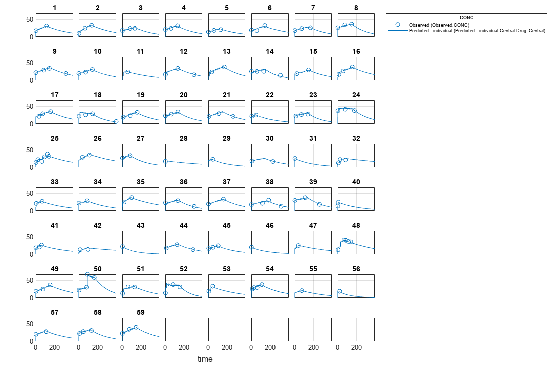
Visualize the fitted results using individual-specific parameter estimates.
plot(nlmeResults,'ParameterType','individual');
Use New Dosing Data to Simulate the Fitted Model
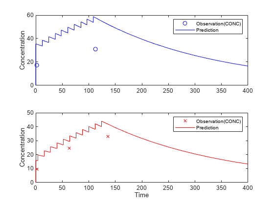
Suppose you want to predict how infants 1 and 2 would have responded under different dosing amounts. You can predict their responses as follows.
Create new dose objects with new dose amounts.
dose1 = doses(1);
dose1.Amount = dose1.Amount*2;
dose2 = doses(2);
dose2.Amount = dose2.Amount*1.5;
Use the predict function to evaluate the fitted model using the new dosing data. If you want response predictions at particular times, provide the new output time vector. Use the 'ParameterType' option to specify individual or population parameters to use. By default, predict uses the population parameters when you specify output times.
timeVec = [0:25:400];
newResults = predict(nlmeResults,timeVec,[dose1;dose2],'ParameterType','population');
Visualize the predicted responses while overlapping the experimental data for infants 1 and 2.
figure;
subplot(2,1,1)
plot(data.TIME(data.ID == 1),data.CONC(data.ID == 1),'bo')
hold on
plot(newResults(1).Time,newResults(1).Data,'b')
hold off
ylabel('Concentration')
legend('Observation(CONC)','Prediction')
subplot(2,1,2)
plot(data.TIME(data.ID == 2),data.CONC(data.ID == 2),'rx')
hold on
plot(newResults(2).Time,newResults(2).Data,'r')
hold off
legend('Observation(CONC)','Prediction')
ylabel('Concentration')
xlabel('Time')
Create a Covariate Model for the Covariate Dependencies
Suppose there is a correlation between volume and weight, and possibly volume and APGAR score. Consider the effect of weight by modeling two of these covariate dependencies: the volume of central (Central) and the clearance rate (Cl_Central) vary with weight. The model becomes
and
Use the CovariateModel object to define the covariate dependencies. For details, see Specify a Covariate Model.
covModel = CovariateModel;
covModel.Expression = ({'Central = exp(theta1 + theta2*WEIGHT + eta1)',...
                        'Cl_Central = exp(theta3 + theta4*WEIGHT + eta2)'});
Use constructDefaultInitialEstimate to create an initialEstimates struct.
initialEstimates = covModel.constructDefaultFixedEffectValues;
Use the FixedEffectNames property to display the thetas (fixed effects) defined in the model.
covModel.FixedEffectNames
ans = 4×1 cell
    {'theta1'}
    {'theta3'}
    {'theta2'}
    {'theta4'}
Use the FixedEffectDescription property to show the descriptions of corresponding fixed effects (thetas) used in the covariate expression. For example, theta2 is the fixed effect for the weight covariate that correlates with the volume (Central), denoted as 'Central/WEIGHT'.
disp('Fixed Effects Description:');Fixed Effects Description:
disp(covModel.FixedEffectDescription);
    {'Central'          }
    {'Cl_Central'       }
    {'Central/WEIGHT'   }
    {'Cl_Central/WEIGHT'}
Set the initial guesses for the fixed-effect parameter values for Central and Cl_Central using the values estimated from fitting the base model.
initialEstimates.theta1 = nlmeResults.FixedEffects.Estimate(1);
initialEstimates.theta3 = nlmeResults.FixedEffects.Estimate(2);
covModel.FixedEffectValues = initialEstimates;
Fit the Model
nlmeResults_cov = sbiofitmixed(onecomp,data,responseMap,covModel,doses,'nlmefit');Display Fitted Parameters and Covariances
disp('Estimated Fixed Effects:');Estimated Fixed Effects:
disp(nlmeResults_cov.FixedEffects);
       Name            Description         Estimate    StandardError
    __________    _____________________    ________    _____________

    {'theta1'}    {'Central'          }    -0.45664      0.078933
    {'theta3'}    {'Cl_Central'       }     -5.9519        0.1177
    {'theta2'}    {'Central/WEIGHT'   }     0.52948      0.047342
    {'theta4'}    {'Cl_Central/WEIGHT'}     0.61954      0.071386
disp('Estimated Covariance Matrix:');Estimated Covariance Matrix:
disp(nlmeResults_cov.RandomEffectCovarianceMatrix);
              eta1        eta2
            ________    ________

    eta1    0.046503           0
    eta2           0    0.041609
Visualize Results
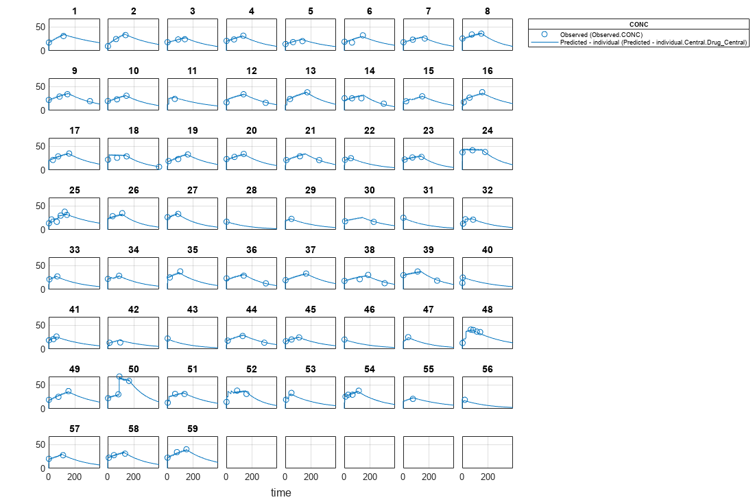
Visualize the fitted results using individual-specific parameter estimates.
plot(nlmeResults_cov,'ParameterType','individual');
Use New Covariate Data to Evaluate the Fitted Model
Suppose you want to explore the responses of infants 1 and 2 using different covariate data, namely WEIGHT. You can do this by specifying the new WEIGHT data. The ID variable of the data corresponds to individual infants.
newData = data(data.ID == 1 | data.ID == 2,:);
newData.WEIGHT(newData.ID == 1) = 1.3;
newData.WEIGHT(newData.ID == 2) = 1.4;
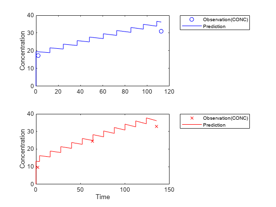
Simulate the responses of infants 1 and 2 using the new covariate data.
[newResults_cov, newEstimates] = predict(nlmeResults_cov,newData,[dose1;dose2]);
newEstimates contains the updated parameter estimates for each individual (infants 1 and 2) after the model is reevaluated using the new covariate data.
newEstimates
newEstimates=4×3 table
    Group         Name         Estimate
    _____    ______________    _________

      1      {'Central'   }       2.5596
      1      {'Cl_Central'}    0.0065965
      2      {'Central'   }       1.7123
      2      {'Cl_Central'}    0.0064806
Compare to the estimated values from the original fit using the old covariate data.
nlmeResults_cov.IndividualParameterEstimates( ...
            nlmeResults_cov.IndividualParameterEstimates.Group == '1' | ...
            nlmeResults_cov.IndividualParameterEstimates.Group == '2',:)
ans=4×3 table
    Group         Name         Estimate
    _____    ______________    _________

      1      {'Central'   }       2.6988
      1      {'Cl_Central'}    0.0070181
      2      {'Central'   }       1.8054
      2      {'Cl_Central'}    0.0068948
Visualize the new simulation results together with the experimental data for infant 1 and 2.
figure;
subplot(2,1,1);
plot(data.TIME(data.ID == 1),data.CONC(data.ID == 1),'bo')
hold on
plot(newResults_cov(1).Time,newResults_cov(1).Data,'b')
hold off
ylabel('Concentration')
legend('Observation(CONC)','Prediction','Location','NorthEastOutside')
subplot(2,1,2)
plot(data.TIME(data.ID == 2),data.CONC(data.ID == 2),'rx')
hold on
plot(newResults_cov(2).Time,newResults_cov(2).Data,'r')
hold off
legend('Observation(CONC)','Prediction','Location','NorthEastOutside')
ylabel('Concentration')
xlabel('Time')
References
[1] Grasela, T. H. Jr., and S. M. Donn. "Neonatal population pharmacokinetics of phenobarbital derived from routine clinical data." Dev Pharmacol Ther 1985:8(6). 374-83.
Input Arguments
Estimation results, specified as a scalar NLMEResults object, which contains nonlinear mixed-effects estimation
results returned by sbiofitmixed.
Grouped data or output times, specified as a groupedData object, vector, or cell array of vectors of output
times.
If data is a groupedData object, it must
have both group labels and output times specified. The group labels can refer to new
groups or existing groups from the original fit. If the mixed-effects model from the
original fit (returned by sbiofitmixed) uses covariates, the
groupedData object must also contain the covariate data with the
same labels for the covariates (CovariateLabels property) specified
in the original CovariateModel object.
By default, individual parameter estimates are used for simulating groups from the
original fit, while population parameters are used for new groups, if any. See the
value argument description for details.
The total number of simulation results in the output ynew
depends on the number of groups or output time vectors in data and
the number of rows in the dosing matrix. For details, see the table
in the ynew argument description.
Dosing information, specified as empty [] or {}, 2-D
matrix or cell vector of SimBiology dose objects (ScheduleDose object or RepeatDose object).
If dosing is empty, no doses are applied during simulation, even if the model has active doses.
For a matrix of dose objects, it must have a single row or one row per group in the input data. If it has a single row, the same doses are applied to all groups during simulation. If it has multiple rows, each row is applied to a separate group, in the same order as the groups appear in the input data. Multiple columns are allowed so that you can apply multiple dose objects to each group.
For a cell vector of doses, it must have one element or one element per group in the input
data. Each element must be [] or a vector of doses. Each element of the
cell is applied to a separate group, in the same order as the groups appear in the input
data.
In addition to manually constructing dose objects using sbiodose, if the input groupedData object has dosing
information, you can use the createDoses method to construct
doses.
Dose objects of the dosing input must be consistent with the original dosing data used with sbiofitmixed. The objects must have the same values for dose properties (such as TargetName) or must be parameterized in the same way as the original dosing data. For instance, suppose that the original dosing matrix has two columns of doses, where the doses in the first column target species x and those in the second column target species y. Then dosing must have doses in the first column targeting species x and those in the second column targeting species y. A parameterized dose example is as follows. Suppose that the Amount property of a dose used in the original sbiofitmixed call is parameterized to a model-scoped parameter 'A'. All doses for the corresponding group (column) in the dosing matrix input must have the Amount property parameterized to 'A'.
The number of rows in the dosing matrix or number of elements in the dosing cell vector and the number of groups or output time vectors in data determine the total number of simulation results in the output ynew. For details, see the table in the ynew argument description.
Note
If UnitConversion is turned on for the underlying SimBiology model that was used for fitting, dosing must specify valid amount and time units.
Name-Value Arguments
Specify optional pairs of arguments as
Name1=Value1,...,NameN=ValueN, where Name is
the argument name and Value is the corresponding value.
Name-value arguments must appear after other arguments, but the order of the
pairs does not matter.
Before R2021a, use commas to separate each name and value, and enclose
Name in quotes.
Example: 'ParameterType','population' specifies to use population
parameter estimates.
Parameter type, specified as 'individual' (default) or
'population'. If value is
'population', the predict method returns the
simulation results using the population parameter estimates, that is, parameter values that are estimated using fixed effects (θs)
only. The estimated parameter values used in simulation are identical to
those in the resultsObj.PopulationParameterEstimates property,
unless you specify a new groupedData object
data with new covariate data. In this case, the method
reevaluates the covariate model and the parameter estimates based on the new
groupedData and covariate data.
If value is 'individual', the method
returns the simulation results using the corresponding parameter values of the group
in the resultsObj.IndividualParameterEstimates property. These
values include both fixed- and random-effects estimates, that is, parameter values estimated using both fixed effects (θs) and
random effects (ηs). If data
contains new groups, only fixed effects (population parameter estimates of the results
object) are used for these groups.
By default, predict uses the individual parameter estimates
of the results object when data is a
groupedData object. If data is a vector of
output times or cell array of vectors, predict uses the
population parameter estimates of the results object instead.
Data Types: char | string
Variants to apply, specified as an empty array ([], {}), 2-D matrix or cell vector of variant objects.
If you do not specify this argument, the function has the following behavior depending on
whether the second input argument (data) is specified also or not.
If
datais not specified, the function applies the group-specific variants from the original call tosbiofitmixed.If
datais a vector or cell array of output times, the function does not apply the group-specific variants.If
datais agroupedDataobject, the function applies variants only to groups whose group identifier matches a group identifier in the original training data that was used in the call tosbiofitmixed.
Note
The baseline variants that were specified by the variants positional input argument in the original call to
sbiofitmixedare always applied to the model, and they are applied before any group-specific variants.If there are no baseline variants, that is, you did not specify the
variantsinput when callingsbiofitmixed, the function still applies the model active variants if there are any.
If the argument value is [] or {}, the function applies no group-specific variants.
If it is a matrix of variants, it must have either one row or one row per group. Each row is
applied to a separate group, in the same order as the groups appear in
data or dosing. If it has a single row, the
same variants are applied to all groups during simulation. If there are multiple columns,
the variants are applied in order from the first column to the last.
If it is a cell vector of variant objects, the number of cells must be one or must match
the number of groups in the input data. Each element must be [] or a
vector of variants. If there is a single cell containing a vector of variants, they are
applied to all simulations. If there are multiple cells, the variants in the
ith cell are applied to the simulation of the ith
group.
The function defines the number of groups by examining the data, and
dosing input arguments.
datacan have1or N groups.If
dataanddosingarguments are not specified, then the default data and dosing are determined as follows:For unpooled fits, they are the data and dosing for the single group associated with that fit results.
For all other fits, they are the entire set of data and dosing associated with the call to
sbiofitmixed.
Output Arguments
Simulation results, returned as a vector of SimData objects. The states reported in ynew are the states included in the responseMap input argument of sbiofitmixed and any other states listed in the StatesToLog property of the runtime options (RuntimeOptions) of the SimBiology model.
The total number of simulation results in ynew depends on the number of groups or output time vectors in data and the number of rows in the dosing matrix.
Number of groups or output time vectors in data | Number of rows in the dosing matrix | Simulation results |
|---|---|---|
|
| The total number of No doses are applied during simulation. |
|
| The total number of The given row of doses is applied during the simulation. |
| N | The total number of Each row of |
N |
| The total number of No doses are applied during simulation. |
N |
| The total number of The same row of doses is applied to each simulation. |
| N | N | The total number of Each row of |
| M | N | The function throws an error when M ≠ N. |
Estimated parameter values used for the predicted simulation results, returned as a table.
If 'ParameterType' is 'individual', the
reported parameter values are identical to the values in the
resultsObj.IndividualParameterEstimates property. However, if
data contains new groups, then only population parameter
estimates (fixed effects) are used for these groups. The corresponding reported values
in parameterEstimates for these groups are identical to the values
in resultsObj.PopulationParameterEstimates.
If 'ParameterType' is 'population', the
reported parameter values are identical to the values in the
resultsObj.PopulationParameterEstimates property unless you specify
new covariate information in data. See the
value argument description for details.
If data is a vector or a cell array of vectors of output times,
the reported parameter values are identical to the values in
resultsObj.PopulationParameterEstimates. Also, the groups reported
represent the enumeration of simulations performed and are unrelated to group names in
the original fit.
Version History
Introduced in R2014a
MATLAB Command
You clicked a link that corresponds to this MATLAB command:
Run the command by entering it in the MATLAB Command Window. Web browsers do not support MATLAB commands.
Select a Web Site
Choose a web site to get translated content where available and see local events and offers. Based on your location, we recommend that you select: .
You can also select a web site from the following list
How to Get Best Site Performance
Select the China site (in Chinese or English) for best site performance. Other MathWorks country sites are not optimized for visits from your location.
Americas
- América Latina (Español)
- Canada (English)
- United States (English)
Europe
- Belgium (English)
- Denmark (English)
- Deutschland (Deutsch)
- España (Español)
- Finland (English)
- France (Français)
- Ireland (English)
- Italia (Italiano)
- Luxembourg (English)
- Netherlands (English)
- Norway (English)
- Österreich (Deutsch)
- Portugal (English)
- Sweden (English)
- Switzerland
- United Kingdom (English)