Create Labeled Signal Sets Iteratively with Reduced Human Effort
This example presents an iterative deep learning-based workflow to label signals with reduced human labeling effort.
Labeling signal data is a tedious and expensive task that requires much human effort. Finding ways to reduce this effort can significantly speed up the development of deep learning solutions for signal processing problems.
Consider the task of labeling regions of interest in a signal data set. A first approach consists of labeling all the data by hand. This approach requires much time and effort. An alternative approach, explored in this example, treats the labeling process iteratively. At each iteration, a subset of signals is selected from the unlabeled data set and is sent to a pretrained deep network for automated labeling. A human labeler examines the resulting labels and corrects wrong labels. The validated labeled signals are added to a training data set to retrain the deep network with the extended training data.
At each iteration, the human labeler still has to visit and examine all the signals labeled by the network. However, the task changes from labeling signals from scratch to correcting inaccurate labels generated by a reliable network. This latter task requires considerably less human labeling effort. At each new iteration, the network is trained with more and more data, causing the prediction and labeling performance of the network to improve. Hence, at each iteration, less and less human intervention is required to correct labels.
This example follows the procedure presented in Waveform Segmentation Using Deep Learning to train a long short-term memory (LSTM) network that can classify ECG signal samples as belonging to one of the three regions of interest.
Data
This example considers the labeling of ECG signal regions using data publicly available in the QT Database [1] [2]. The data consists of roughly 15 minutes of ECG recordings from a total of 105 patients. To obtain each recording, the examiners placed two electrodes on different locations on a patient's chest, resulting in a two-channel signal. The database provides signal region labels generated by an automated expert system [3]. The labels correspond to the locations of P wave, T wave, and QRS complex regions in the ECG measurements. Each channel of the 105 two-channel ECG signals was labeled independently by the automated expert system and is treated independently for a total of 210 ECG signals that were stored together with the region labels in 210 MAT files. The files are available at the following location: https://www.mathworks.com/supportfiles/SPT/data/QTDatabaseECGData1.zip.
Download the dataset using the downloadSupportFile function.
% Download the data
datasetZipFile = matlab.internal.examples.downloadSupportFile('SPT','data/QTDatabaseECGData1.zip');
datasetFolder = fullfile(fileparts(datasetZipFile),'QTDataset');
if ~exist(datasetFolder,'dir')
     unzip(datasetZipFile,fileparts(datasetZipFile));
end
The unzip operation creates the datasetFolder folder with 210 MAT files in it. Each file contains an ECG signal in variable ecgSignal and a table of region labels in variable signalRegionLabels. Each file also contains the sample rate of the signal in variable Fs. In this example all signals have a sample rate of 250 Hz.
Create a signal datastore to access the data in the files. Specify the signal variable names you want to read from each file using the SignalVariableNames parameter.
sds = signalDatastore(datasetFolder,'SignalVariableNames',["ecgSignal","signalRegionLabels"]);
The datastore returns a two-element cell array with an ECG signal and a table of region labels each time you call the read function. Use the preview function of the datastore to see that the content of the first file is a 225,000 samples long ECG signal and a table containing 3385 region labels.
data = preview(sds)
data=2×1 cell array
    225000×1 double
       3385×2 table
Look at the first few rows of the region labels table and observe that each row contains the region limit indices and the region class value (P, T, or QRS).
head(data{2}) ROILimits Value
__________ _____
83 117 P
130 153 QRS
201 246 T
285 319 P
332 357 QRS
412 457 T
477 507 P
524 547 QRS
Visualize the labels for the first 1000 samples using a signalMask object.
MGroundTruth = signalMask(data{2});
plotsigroi(MGroundTruth,data{1}(1:1000))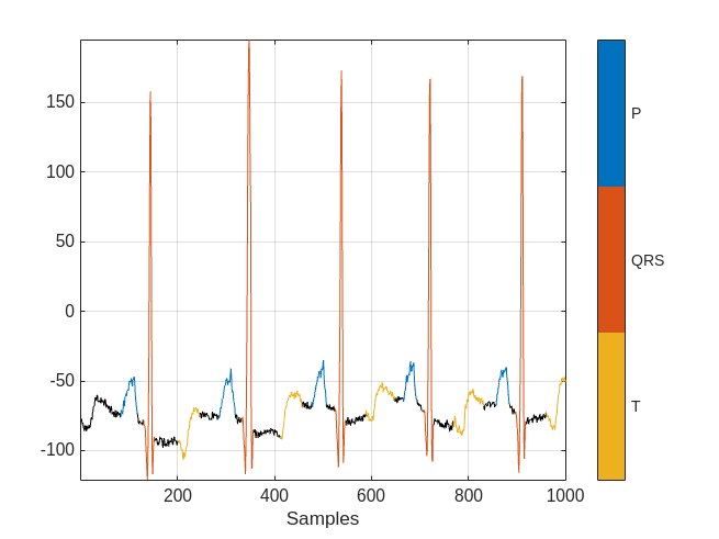
Convert the region-of-interest labels to a categorical sequence to be able to train a deep network to perform sequence-to-sequence classification. Use the transform function of the datastore to apply the transformation when the signal data is read from disk.
numFiles = numel(sds.Files);
sds = transform(sds,@getmask);
Resize (split) the signals and labels to obtain multiple segments of length 5000 samples and convert each ECG segment into the time-frequency domain using the Fourier synchrosqueezed transform (FSST).
sds = transform(sds,@resizeData);
sdsFSST = transform(sds,@(x,fs)extractFSSTFeatures(x,250));
Use 70% of the files for training and 30% for testing. Shuffle the dataset so that the training and testing signals are chosen randomly.
rng default
[trainIdx,~,testIdx] = dividerand(numFiles,0.7,0,0.3);

trainDs = subset(sds,trainIdx); % resized 5000 sample signals and labels
trainDsFSST = subset(sdsFSST,trainIdx); % FSST-transformed signals and labels

testDsFSST = subset(sdsFSST,testIdx);
Read all the data into memory using the readall method of the datastores. This action will read each ECG signal and apply all the transformations described above to return multiple Fourier synchrosqueeze-transformed ECG segments. Use the UseParallel option to transform the dataset in parallel using the available processors in your computer whenever you have Parallel Computing Toolbox™.
% Get FSST-transformed signals
ecgFSSTData = readall(trainDsFSST,UseParallel=true);
Starting parallel pool (parpool) using the 'Processes' profile ... Connected to parallel pool with 8 workers.
testFSSTData = readall(testDsFSST,UseParallel=true);

ecgFSST = ecgFSSTData(:,1);
ecgLabels = ecgFSSTData(:,2);

testECGFSST = testFSSTData(:,1);
testLabels = testFSSTData(:,2);

% Get time domain signal segments so that we can plot some labeling results
ecgData = readall(trainDs);
ecgSignals = ecgData(:,1);
This example shows that it is possible to decrease the human effort involved in signal labeling by iteratively training a deep network. At each iteration:
The network labels a subset of unlabeled data frames using previously labeled frames.
A human labeler corrects any labeling errors by hand.
The corrected labeling is added to the previously labeled frames.
The expanded set of labeled signals is used to train the network for the next iteration.
To make quantitative comparisons, simulate two scenarios:
For the baseline scenario, in which a human labels the entire dataset from scratch, train the network using the full labeled
ecgFramesset.For the second scenario, pretend that the
ecgFramesdata is unlabeled and label it using the iterative method
Prediction Performance Using Fully Labeled ECG Data Set
Build a BiLSTM network and train it with the full labeled ecgFrames set to get a prediction-performance upper bound. As mentioned above, this approach requires brute-force labeling of the whole data set and hence the largest human labeling effort. Train the network with the labeled ecgFrames set and calculate the prediction accuracy on the test data set.
Network Architecture
Create a BiLSTM network using deep learning layers.
Specify a
sequenceInputLayerwith a size as the number of features in the FSST of the signals, which is the total number of frequency-domain samples (40 in this example).Specify a
bilstmLayerwith 200 hidden nodes and set theOutputModetosequencesince each signal sample has a label.Specify a
fullyConnectedLayerwith an output size of 4 corresponding to the four categories, P wave, QRS complex, T wave, and N/A.Add a
softmaxLayerto output the estimated probabilities for each category.
% Training with the full emulated unlabeled data set
layers = [ ...
    sequenceInputLayer(size(ecgFSST{1},2))
    bilstmLayer(200,'OutputMode','sequence')
    fullyConnectedLayer(4)
    softmaxLayer];
Use traningOptions to specify the optimization solver and the hyperparameters to train the network. This example uses the ADAM optimizer and a mini-batch size of 50. Train the network using either a CPU or GPU. Using a GPU requires Parallel Computing Toolbox™. To see which GPUs are supported, see GPU Computing Requirements (Parallel Computing Toolbox). For information on other parameters, see trainingOptions (Deep Learning Toolbox). This example uses a GPU for training using the 'ExecutionEnvironment' name-value pair.
options = trainingOptions('adam', ...
    'MaxEpochs',10, ...
    'MiniBatchSize',50, ...
    'ExecutionEnvironment','gpu', ...
    'InitialLearnRate',0.01, ...
    'LearnRateDropPeriod',6, ...
    'LearnRateSchedule','piecewise', ...
    'GradientThreshold',1, ...
    'Shuffle','every-epoch',...
    'Plots','training-progress',...
    'Verbose',0,...
    'Metric','Accuracy');
Train the network with the fully labeled ecgFrames data set.
baselineNet = trainnet(ecgFSST,ecgLabels,layers,"crossentropy",options);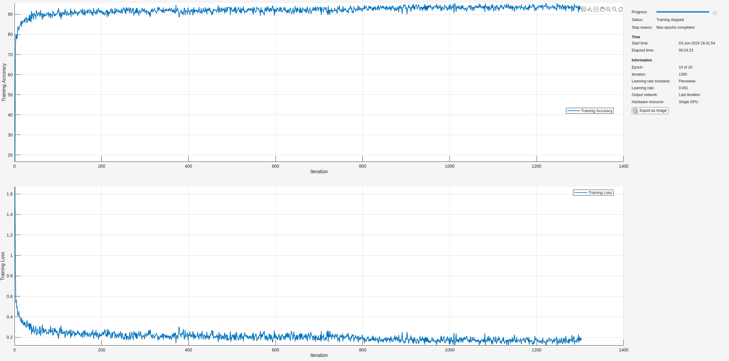
Classify the test frames using the trained network and compute the mean prediction accuracy. The baseline prediction accuracy is about 90%.
scores = minibatchpredict(baselineNet,testECGFSST);
classNames = categories(ecgLabels{1});
predictLabelsAll = squeeze(mat2cell(scores2label(scores,classNames),size(scores,1),1,ones(size(scores,3),1)));
accuracyAll = mean(cellfun(@(x,y)mean(x==y),predictLabelsAll,testLabels));
fprintf('The baseline prediction accuracy is %2.1f%%.\n',accuracyAll*100);
The baseline prediction accuracy is 89.6%.
Iterative Labeling with Human in the Loop
To reduce the labeling effort, try an iterative approach: Pretend that the ecgFrames data set is initially unlabeled and that the data are labeled manually. In reality, the example uses the ground truth labels provided by the data set.
Train an Initial Network
Start by selecting 25 frames from the ecgFrames set and labeling them manually. Train a BiLSTM network with this initial labeled set to serve as the initial step of the iterative process.
numInitFrames = 25;

currentTrainingSet = ecgFSST(1:numInitFrames,1);
currentTrainingLabels = ecgLabels(1:numInitFrames);
Set the training options to have more training epochs and a smaller mini-batch size because there are only 25 frames within the initial training data set.
options = trainingOptions('adam', ...
    'MaxEpochs',20, ...
    'MiniBatchSize',5, ...
    'ExecutionEnvironment','gpu', ...
    'InitialLearnRate',0.01, ...
    'LearnRateDropPeriod',6, ...
    'LearnRateSchedule','piecewise', ...
    'GradientThreshold',1, ...
    'Shuffle','every-epoch', ...
    'Plots','none',...
    'Verbose',0);
Train the BiLSTM network with the initial training data set and predict labels using the same test data set used to establish the performance baseline. The prediction accuracy of this initial network is around 40%.
initNet = trainnet(currentTrainingSet,currentTrainingLabels,layers,"crossentropy",options);scores = minibatchpredict(initNet,testECGFSST,'MiniBatchSize',50); initPrediction = squeeze(mat2cell(scores2label(scores,classNames),size(scores,1),1,ones(size(scores,3),1))); initAccuracy = mean(cellfun(@(x,y)mean(x==y),initPrediction,testLabels)); fprintf('The prediction accuracy is %2.1f%%.\n',initAccuracy*100);
The prediction accuracy is 40.2%.
Labeling
In the next step, select 200 new data frames from the ecgFrames set and feed them to the pretrained network, initNet, to label the signals automatically.
iteration = 1;
% Number of frames to label at each iteration
numFrames = 200;
% Select the next set of frames to label
indexNext = numInitFrames+1:numInitFrames+numFrames;
% Use classify to label the new frames
scores = minibatchpredict(initNet,ecgFSST(indexNext),'MiniBatchSize',50);
currentPrediction = squeeze(mat2cell(scores2label(scores,classNames),size(scores,1),1,ones(size(scores,3),1)));
Evaluate the labeling results generated by the network and compare them to the ground truth. Find the indices of the ECG signals that got the best- and worst-case performance with this network.
errs = cellfun(@(x,y)sum(x~=y),ecgLabels(indexNext),currentPrediction);
[~,bestIndex] = min(errs);
[~,worstIndex] = max(errs);
For the best-case scenario, plot the first 750 samples overlaid with the ground-truth labels and the labels predicted by the network.
ecgSignalOfInterest = ecgSignals{indexNext(bestIndex)};
groundTruthLabels = ecgLabels{indexNext(bestIndex)};
predictedLabels = currentPrediction{bestIndex};

MGroundTruth = signalMask(groundTruthLabels);
figure
plotsigroi(MGroundTruth,ecgSignalOfInterest(1:750))
title('Ground Truth - best-case scenario')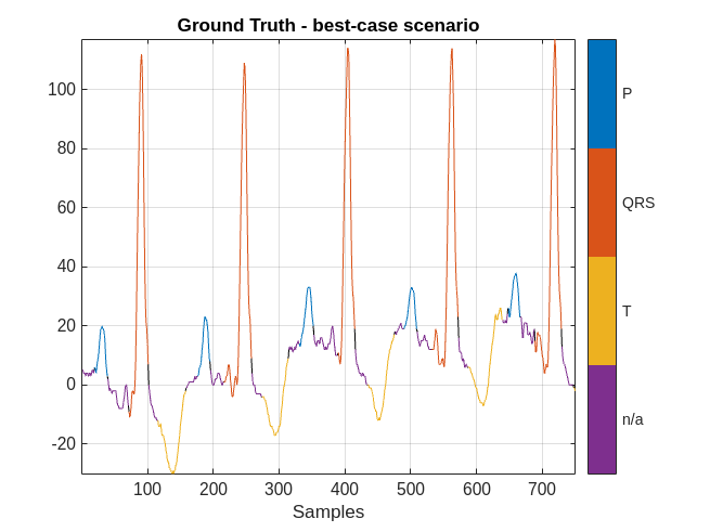
MPredicted = signalMask(predictedLabels);
figure
plotsigroi(MPredicted,ecgSignalOfInterest(1:750))
title('Labeling by Network - best-case scenario')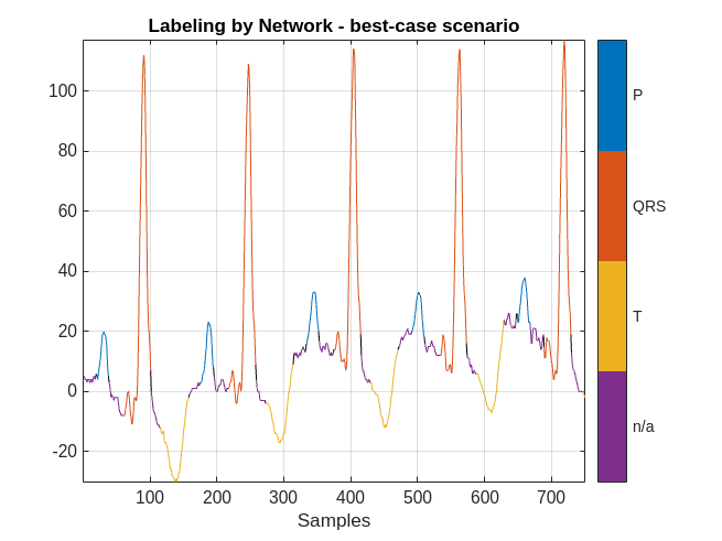
The network did a good job labeling this frame. As a result, a human inspecting the results of the network can correct the predicted labels with little effort.
However, there are cases when the labeling performance of the network is not as strong. Plot the results obtained in the worst-case scenario.
ecgSignalOfInterest = ecgSignals{indexNext(worstIndex)};
groundTruthLabels = ecgLabels{indexNext(worstIndex)};
predictedLabels = currentPrediction{worstIndex};

MGroundTruth = signalMask(groundTruthLabels);
figure
plotsigroi(MGroundTruth,ecgSignalOfInterest(1:750))
title('Ground Truth - worst-case scenario')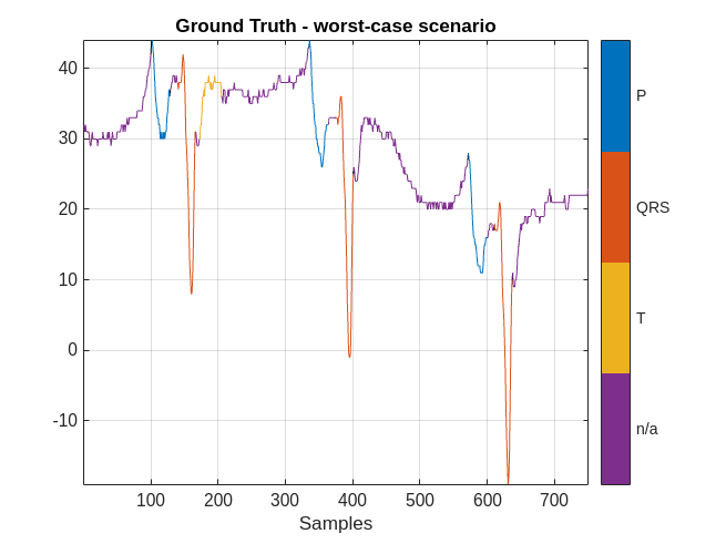
MPredicted = signalMask(predictedLabels);
figure
plotsigroi(MPredicted,ecgSignalOfInterest(1:750))
title('Labeling by Network - worst-case scenario')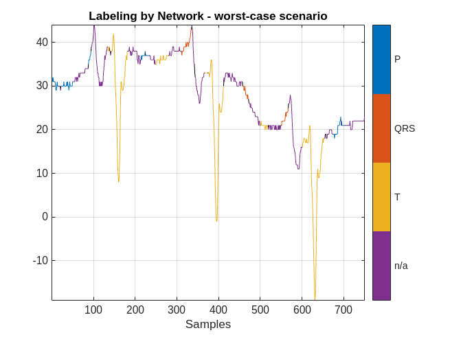
The performance of the network on this signal is not as good. In this case, a human labeler has to make several corrections to the predicted labels.
To quantify the correction effort for the 200 data frames, calculate the labeling error rate of the network and the average number of samples per frame that must be corrected by the human labeler.
numSamplesPerFrame = 5000;
networkLabelingErrorRate(iteration) = 1-mean(cellfun(@(x,y)mean(x==y),currentPrediction,ecgLabels(indexNext)));
averageNumOfCorrectionsPerFrame(iteration) = networkLabelingErrorRate(iteration) * numSamplesPerFrame;
fprintf('The average number of corrections per frame is %2.1f.\n',averageNumOfCorrectionsPerFrame(iteration));
The average number of corrections per frame is 2374.6.
For the first iteration, there are on average about 2200 samples per frame that must be corrected by a human. Corrected samples per frame is a convenient metric to show human effort. Note however that in practice, a human labeler does not have to correct the label of each sample. Instead, the human labeler only has to extend or shorten region limits.
At the end of the first iteration, the human will inspect the 200 frames and modify any label with incorrect values. With the help of the network and the human labeler, the data frames have correct labels at the end of the iteration.
On the next iteration, the 200 newly labeled frames can be added to the currentTrainingSet set to retrain the network and repeat the labeling iteration. This chart illustrates the workflow in each iteration after the first iteration:
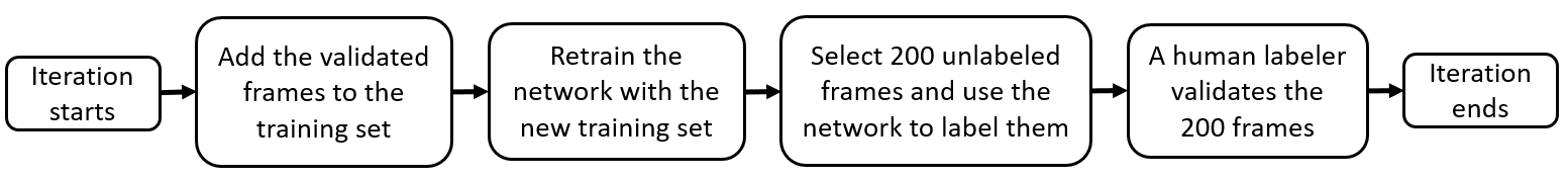
Repeat Labeling Iterations
Extend the training set by adding the newly corrected labeled frames, select another 200 data frames to be labeled, and repeat the labeling iteration until the performance is satisfactory.
% Include the initial training set and the 200 newly labeled data frames
maxIter = 15;
indexTraining = 1:numInitFrames+numFrames;

networkAccuracy = zeros(1,15);
networkAccuracy(iteration) = initAccuracy;

options = trainingOptions('adam', ...
    'MaxEpochs',20, ...
    'MiniBatchSize',50, ...
    'ExecutionEnvironment','gpu', ...
    'InitialLearnRate',0.01, ...
    'LearnRateDropPeriod',6, ...
    'LearnRateSchedule','piecewise', ...
    'GradientThreshold',1, ...
    'Shuffle','every-epoch', ...
    'Plots','none', ...
    'Verbose',0);

for iteration = 2:maxIter
    % Extended training data set
    currentTrainingSet = ecgFSST(indexTraining,1);
    % Emulate human correction by assigning ground-truth labels to the
    % extended training set
    currentTrainingLabels = ecgLabels(indexTraining);

    % Train network with extended training set
    currentNet = trainnet(currentTrainingSet,currentTrainingLabels,layers,"crossentropy",options);

    % Predict labels for the test data set and calculate the accuracy to
    % compare to baseline performance
    scores = minibatchpredict(currentNet,testECGFSST,'MiniBatchSize',50);
    currentTestSetPrediction = squeeze(mat2cell(scores2label(scores,classNames),size(scores,1),1,ones(size(scores,3),1)));
    networkAccuracy(iteration) = mean(cellfun(@(x,y)mean(x==y),currentTestSetPrediction,testLabels));

    % Get another numFrames data frames for human labeler
    indexNext = indexTraining(end)+1:indexTraining(end)+numFrames;

    % Measure average number of human corrections per frame in this iteration
    scores = minibatchpredict(currentNet,ecgFSST(indexNext),'MiniBatchSize',50);
    currentPrediction = squeeze(mat2cell(scores2label(scores,classNames),size(scores,1),1,ones(size(scores,3),1)));
    networkLabelingErrorRate(iteration) = 1-mean(cellfun(@(x,y)mean(x==y),currentPrediction,ecgLabels(indexNext)));
    averageNumOfCorrectionsPerFrame(iteration) = networkLabelingErrorRate(iteration) * numSamplesPerFrame;

    indexTraining = 1:indexNext(end);
end
Labeling Performance
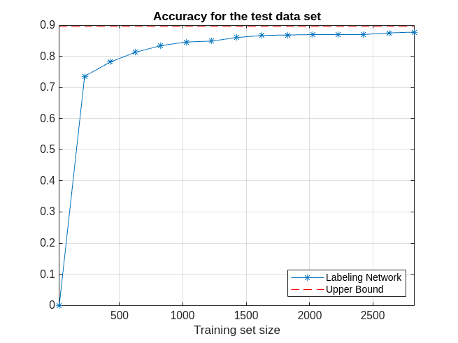
After 15 labeling iterations, there are 2825 data frames in currentTrainingSet, corresponding to about half of the 6543 data frames contained in the full ecgDataset set. The prediction accuracy of the network trained with 2825 frames is already very close to the baseline accuracy.
accuDiff = accuracyAll-networkAccuracy(end);
fprintf('The accuracy difference is %2.1f%%.\n',accuDiff*100);
The accuracy difference is 1.8%.
Plot the network prediction accuracy for the test data set with respect to the size of the training data set at each iteration. Show the upper bound of the accuracy obtained with the fully labeled data set. As more data frames are validated, the prediction accuracy of the network improves.
figure
examinedDataSize = 25:200:2825;
plot(examinedDataSize,networkAccuracy,'*-')
hold on
% Prediction accuracy upper bound
plot(examinedDataSize,ones(1,15)*accuracyAll,'r--')
grid on
xlabel('Training set size')
title('Accuracy for the test data set')
xlim([25 2825])
legend('Labeling Network','Upper Bound','Location','southeast')
As iterations progress, the average number of human corrections per frame decreases as the size of the training dataset increases. As more data frames are validated and used to train the network, less human effort is required to correct the labels of the selected frames.
figure
plot(examinedDataSize,averageNumOfCorrectionsPerFrame,'*-')
grid on
xlabel('Training set size')
title('Average number of human corrections per frame')
xlim([25 2825])

Throughout all 15 labeling iterations, an average of about 700 signal samples per frame required human corrections. As mentioned earlier, in practice, a human corrects labeled regions by extending or shortening region limits and not by changing individual sample labels.
fprintf('The average number of corrections per frame is %2.1f.\n',mean(averageNumOfCorrectionsPerFrame));The average number of corrections per frame is 727.9.
Conclusion
This example showed that labeling only half of an ECG data set allows a deep network to achieve a prediction accuracy similar to that achieved by the same network when trained with the fully labeled data set. With the proposed iterative labeling workflow, a human labeler needs to look at only half of the data set and correct an average of 700 signal samples per frame. On the other hand, brute-force labeling requires looking at every frame in the data set and labeling all of its samples from scratch.
References
[1] Goldberger, Ary L., Luis A. N. Amaral, Leon Glass, Jeffery M. Hausdorff, Plamen Ch. Ivanov, Roger G. Mark, Joseph E. Mietus, George B. Moody, Chung-Kang Peng, and H. Eugene Stanley. "PhysioBank, PhysioToolkit, and PhysioNet: Components of a New Research Resource for Complex Physiologic Signals." Circulation. Vol. 101, Number 23, 2000, pp. e215–e220. [Circulation Electronic Pages; http://circ.ahajournals.org/content/101/23/e215.full].
[2] Laguna, Pablo, Roger G. Mark, Ary L. Goldberger, and George B. Moody. "A Database for Evaluation of Algorithms for Measurement of QT and Other Waveform Intervals in the ECG." Computers in Cardiology. Vol.24, 1997, pp. 673–676.
[3] Laguna, Pablo, Raimon Jané, and Pere Caminal. "Automatic detection of wave boundaries in multilead ECG signals: Validation with the CSE database." Computers and Biomedical Research. Vol. 27, Number 1, 1994, pp. 45–60.