Frequency Response
Digital Domain
freqz uses an FFT-based
algorithm to calculate the Z-transform frequency response of a digital
filter. Specifically, the statement
[h,w] = freqz(b,a,p)
returns the p-point complex frequency response, H(ejω), of the digital filter.
In its simplest form, freqz accepts the filter
coefficient vectors b and a,
and an integer p specifying the number of points
at which to calculate the frequency response. freqz returns
the complex frequency response in vector h, and
the actual frequency points in vector w in rad/s.
freqz can accept other parameters, such as
a sampling frequency or a vector of arbitrary frequency points. The
example below finds the 256-point frequency response for a 12th-order
Chebyshev Type I filter. The call to freqz specifies
a sampling frequency fs of 1000 Hz:
[b,a] = cheby1(12,0.5,200/500);
[h,f] = freqz(b,a,256,1000);
Because the parameter list includes a sampling frequency, freqz returns
a vector f that contains the 256 frequency points
between 0 and fs/2 used in the frequency response
calculation.
Note
This toolbox uses the convention that unit frequency is the Nyquist frequency, defined as half the sampling frequency. The cutoff frequency parameter for all basic filter design functions is normalized by the Nyquist frequency. For a system with a 1000 Hz sampling frequency, for example, 300 Hz is 300/500 = 0.6. To convert normalized frequency to angular frequency around the unit circle, multiply by π. To convert normalized frequency back to hertz, multiply by half the sample frequency.
If you call freqz with no output arguments,
it plots both magnitude versus frequency and phase versus frequency.
For example, a ninth-order Butterworth lowpass filter with a cutoff
frequency of 400 Hz, based on a 2000 Hz sampling frequency, is
[b,a] = butter(9,400/1000);
To calculate the 256-point complex frequency response for this
filter, and plot the magnitude and phase with freqz,
use
freqz(b,a,256,2000)
freqz can also accept a vector of arbitrary
frequency points for use in the frequency response calculation. For
example,
w = linspace(0,pi);
h = freqz(b,a,w);
calculates the complex frequency response at the frequency points
in w for the filter defined by
vectors b and a.
The frequency points can range from 0 to 2π.
To specify a frequency vector that ranges from zero to your sampling
frequency, include both the frequency vector and the sampling frequency
value in the parameter list.
These examples show how to compute and display digital frequency responses.
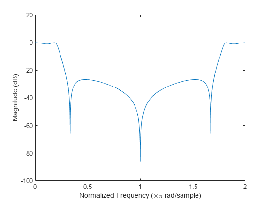
Frequency Response from Transfer Function
Compute and display the magnitude response of the third-order IIR lowpass filter described by the following transfer function:
Express the numerator and denominator as polynomial convolutions. Find the frequency response at 2001 points spanning the complete unit circle.
b0 = 0.05634;
b1 = [1  1];
b2 = [1 -1.0166 1];
a1 = [1 -0.683];
a2 = [1 -1.4461 0.7957];

b = b0*conv(b1,b2);
a = conv(a1,a2);

[h,w] = freqz(b,a,"whole",2001);
Plot the magnitude response expressed in decibels.
plot(w/pi,20*log10(abs(h)))
ax = gca;
ax.YLim = [-100 20];
ax.XTick = 0:.5:2;
xlabel("Normalized Frequency (\times\pi rad/sample)")
ylabel("Magnitude (dB)")
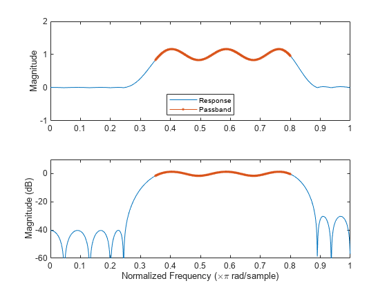
Frequency Response of an FIR Bandpass Filter
Design an FIR bandpass filter with passband between and rad/sample and 3 dB of ripple. The first stopband goes from to rad/sample and has an attenuation of 40 dB. The second stopband goes from rad/sample to the Nyquist frequency and has an attenuation of 30 dB. Compute the frequency response. Plot its magnitude in both linear units and decibels. Highlight the passband.
sf1 = 0.1;
pf1 = 0.35;
pf2 = 0.8;
sf2 = 0.9;
pb = linspace(pf1,pf2,1e3)*pi;

bp = designfilt("bandpassfir", ...
    StopbandAttenuation1=40,StopbandFrequency1=sf1, ...
    PassbandFrequency1=pf1,PassbandRipple=3, ...
    PassbandFrequency2=pf2,StopbandFrequency2=sf2, ...
    StopbandAttenuation2=30);

[h,w] = freqz(bp,1024);
hpb = freqz(bp,pb);

subplot(2,1,1)
plot(w/pi,abs(h),pb/pi,abs(hpb),'.-')
axis([0 1 -1 2])
legend("Response","Passband",Location="south")
ylabel("Magnitude")

subplot(2,1,2)
plot(w/pi,db(h),pb/pi,db(hpb),".-")
axis([0 1 -60 10])
xlabel("Normalized Frequency (\times\pi rad/sample)")
ylabel("Magnitude (dB)")
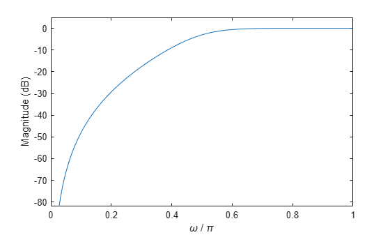
Magnitude Response of a Highpass Filter
Design a 3rd-order highpass Butterworth filter having a normalized 3 dB frequency of rad/sample. Compute its frequency response. Express the magnitude response in decibels and plot it.
[b,a] = butter(3,0.5,"high");
[h,w] = freqz(b,a);

dB = mag2db(abs(h));

plot(w/pi,dB)
xlabel("\omega / \pi")
ylabel("Magnitude (dB)")
ylim([-82 5])
Analog Domain
freqs evaluates frequency
response for an analog filter defined by two input coefficient vectors, b and a. Its operation is similar to that
of freqz; you can specify a number of frequency
points to use, supply a vector of arbitrary frequency points, and
plot the magnitude and phase response of the filter. This example
shows how to compute and display analog frequency responses.
Comparison of Analog IIR Lowpass Filters
Design a fifth-order analog Butterworth lowpass filter with a cutoff frequency of 2 GHz. Multiply by to convert the frequency to radians per second. Compute the frequency response of the filter at 4096 points.
n = 5;
wn = 2*pi*2e9;
w = 2*pi*1e9*logspace(-2,1,4096)';

[zb,pb,kb] = butter(n,wn,"s");
[bb,ab] = zp2tf(zb,pb,kb);
[hb,wb] = freqs(bb,ab,w);
gdb = -diff(unwrap(angle(hb)))./diff(wb);
Design a fifth-order Chebyshev Type I filter with a passband edge frequency of 2 GHz and 3 dB of passband ripple. Compute its frequency response.
wp = wn;

[z1,p1,k1] = cheby1(n,3,wp,"s");
[b1,a1] = zp2tf(z1,p1,k1);
[h1,w1] = freqs(b1,a1,w);
gd1 = -diff(unwrap(angle(h1)))./diff(w1);
Design a fifth-order Chebyshev Type II filter with a stopband edge frequency of 2.5 GHz and 30 dB of stopband attenuation. Compute its frequency response.
ws = 2*pi*2.5e9;

[z2,p2,k2] = cheby2(n,30,ws,"s");
[b2,a2] = zp2tf(z2,p2,k2);
[h2,w2] = freqs(b2,a2,w);
gd2 = -diff(unwrap(angle(h2)))./diff(w2);
Design a fifth-order elliptic filter with the same passband and stopband edge frequencies, 3 dB of passband ripple, and 30 dB of stopband attenuation. Compute its frequency response.
[ze,pe,ke] = ellip(n,3,30,wp,"s");
[be,ae] = zp2tf(ze,pe,ke);
[he,we] = freqs(be,ae,w);
gde = -diff(unwrap(angle(he)))./diff(we);
Design a fifth-order Bessel filter with the same edge frequency. Compute its frequency response.
[zf,pf,kf] = besself(n,wn);
[bf,af] = zp2tf(zf,pf,kf);
[hf,wf] = freqs(bf,af,w);
gdf = -diff(unwrap(angle(hf)))./diff(wf);
Plot the attenuation in decibels. Express the frequency in gigahertz. Compare the filters.
fGHz = [wb w1 w2 we wf]/(2e9*pi);
plot(fGHz,mag2db(abs([hb h1 h2 he hf])))
axis([0 5 -45 5])
grid on
xlabel("Frequency (GHz)")
ylabel("Attenuation (dB)")
legend(["butter" "cheby1" "cheby2" "ellip" "besself"], ...
    Location="southwest")

The Butterworth and Chebyshev Type II filters have flat passbands and wide transition bands. The Chebyshev Type I and elliptic filters roll off faster but have passband ripple. The frequency input to the Chebyshev Type II design function sets the beginning of the stopband rather than the end of the passband. Elliptic filters offer steeper rolloff characteristics than Butterworth and Chebyshev filters, but they are equiripple in both the passband and the stopband. Of these four classical filter types, elliptic filters usually meet a given set of filter performance specifications with the lowest filter order.
Plot the group delay in samples. Express the frequency in gigahertz and the group delay in nanoseconds. Compare the filters. The Bessel filter has approximately constant group delay along the passband.
gdns = [gdb gd1 gd2 gde gdf]*1e9;
gdns(gdns<0) = NaN;
loglog(fGHz(2:end,:),gdns)
grid on
xlabel("Frequency (GHz)")
ylabel("Group delay (ns)")
legend(["butter" "cheby1" "cheby2" "ellip" "besself"], ...
    Location="southwest")
