Use Filter Analyzer App
App Workflow
A typical workflow for designing filters using the Filter Analyzer app is:
Import Filters and Manage Sessions — Import existing filters available in the MATLAB® workspace, where each filter is either a set of numeric variables, a
digitalFilterobject, or one of the supported filter System objects (DSP System Toolbox) from DSP System Toolbox™. You can also save and share your Filter Analyzer session.Manage and Analyze Filters — View and compare filter details, analyze filter responses in frequency and time domains, organize analysis with multiple displays and display options.
Example: Analyze Lowpass IIR Filter
Use the Filter Analyzer app to import and analyze a lowpass filter that preserves frequency content under 200 Hz for signals sampled at 1 kHz. Use the Chebyshev type II filter design to create a low-order filter with a narrow transition region and no ripple in the passband.
Create Filter
Use the designfilt function to create a fifth-order Chebyshev type II filter with a sample rate of 1 kHz. You can also Use Filter Designer App to create the filter.
d = designfilt("lowpassiir",SampleRate=1000, ...
    FilterOrder=5,StopbandFrequency=200,ScaleSOS=true);
Import Filter
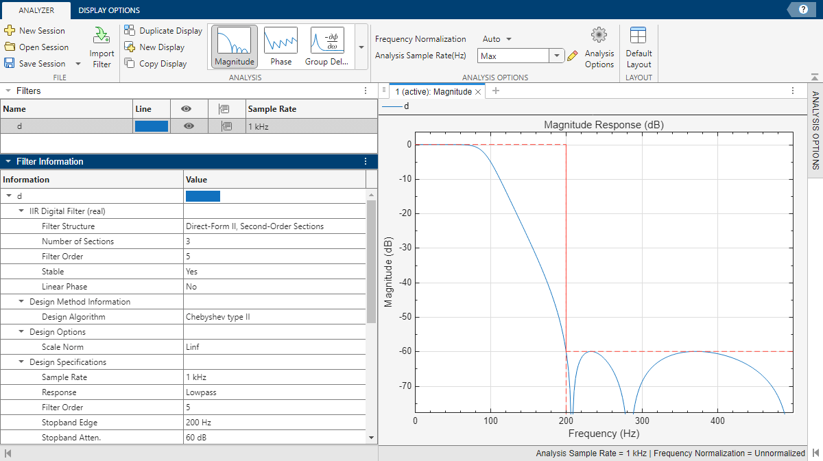
Open Filter Analyzer. In the File section of the Analyzer tab in the app toolstrip, select Import Filter. In the dialog box that appears, select the digitalFilter object d and click Import and Close. The app displays a filter design with the expected design specifications.
Inspect Filter
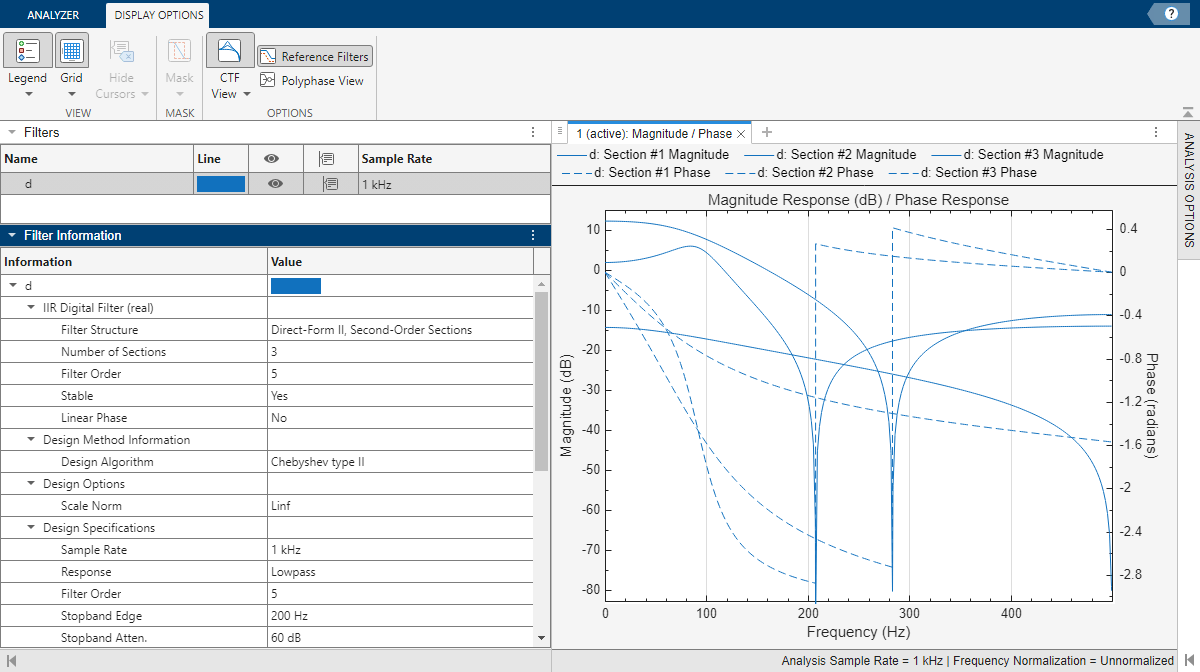
To inspect the filter, plot the magnitude and phase responses and set display options.
Add the phase response as an overlaid analysis to the active display. In the Analysis gallery in the Analyzer tab, select
Phaseunder Overlay Analysis.Show the CTF sections of the filter. In the Display Options tab, click CTF View.