rainflow

Rainflow counts for fatigue analysis

Syntax

c = rainflow(x)

c = rainflow(x,fs)

c = rainflow(x,t)

c = rainflow(xt)

c = rainflow(___,'ext')

[c,rm,rmr,rmm] = rainflow(___)

[c,rm,rmr,rmm,idx] = rainflow(___)

rainflow(___)

Description

c = rainflow(x) returns cycle counts for the load time history, x, according to the ASTM E 1049 standard. See Algorithms for more information.

c = rainflow(x,fs) returns cycle counts for x sampled at a rate fs.

c = rainflow(x,t) returns cycle counts for x sampled at the time values stored in t.

c = rainflow(xt) returns cycle counts for the time history stored in the MATLAB^® timetable xt.

c = rainflow(___,'ext') specifies the time history as a vector of identified reversals (peaks and valleys). 'ext' can be used with any of the previous syntaxes.

[c,rm,rmr,rmm] = rainflow(___) outputs a rainflow matrix, rm, and two vectors, rmr and rmm, containing histogram bin edges for the rows and columns of rm, respectively.

[c,rm,rmr,rmm,idx] = rainflow(___) also returns the linear indices of the reversals identified in the input.

rainflow(___) with no output arguments plots load reversals and a rainflow matrix histogram in the current figure.

Examples

Cycle Counts with Known Sample Rate

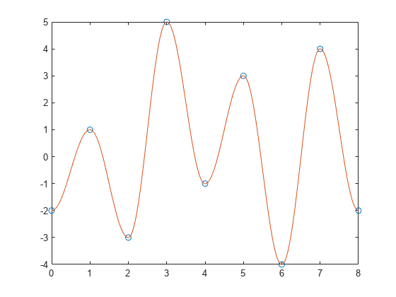
Generate a signal that resembles a load history, consisting of sinusoid half-periods connecting known, equispaced reversals. The signal is sampled at 512 Hz for 8 seconds. Plot the extrema and the signal.

fs = 512;

X = [-2 1 -3 5 -1 3 -4 4 -2];
lX = length(X)-1;

Y = -diff(X)/2.*cos(pi*(0:1/fs:1-1/fs)') + (X(1:lX)+X(2:lX+1))/2;
Y = [Y(:);X(end)];

plot(0:lX,X,"o",0:1/fs:lX,Y)

Compute cycle counts for the data. Display the matrix of cycle counts.

[c,hist,edges,rmm,idx] = rainflow(Y,fs);

T = array2table(c,VariableNames=["Count" "Range" "Mean" "Start" "End"])

T=7×5 table
    Count    Range    Mean    Start    End
    _____    _____    ____    _____    ___

     0.5       3      -0.5      0       1 
     0.5       4        -1      1       2 
       1       4         1      4       5 
     0.5       8         1      2       3 
     0.5       9       0.5      3       6 
     0.5       8         0      6       7 
     0.5       6         1      7       8 

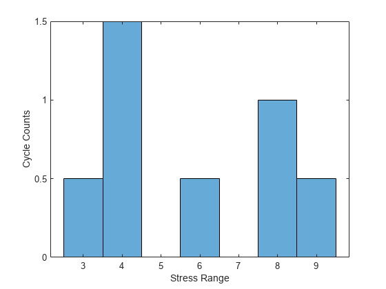
Display a histogram of cycle counts as a function of stress range.

histogram(BinEdges=edges',BinCounts=sum(hist,2))
xlabel("Stress Range")
ylabel("Cycle Counts")

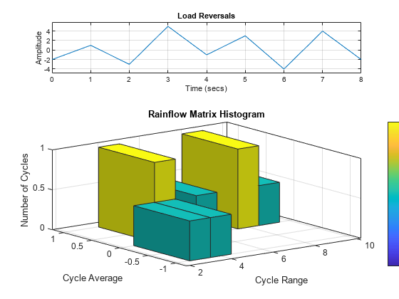
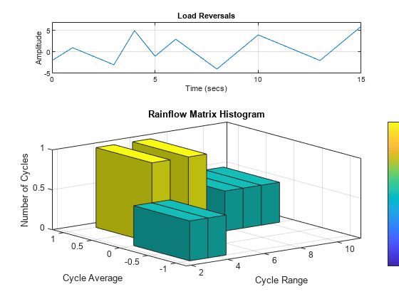
Use rainflow without output arguments to display a histogram of cycles as a function of cycle average and cycle range.

rainflow(Y,fs)

Cycle Counts with Known Time Values

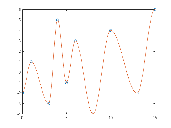
Generate a signal that resembles a load history, consisting of sinusoid half-periods connecting known, unevenly spaced reversals. The signal is sampled at 10 Hz for 15 seconds. Plot the extrema and the signal.

fs = 10;

X = [0 1 3 4 5 6 8 10 13 15];
Y = [-2 1 -3 5 -1 3 -4 4 -2 6];

Z = [];
for k = 1:length(Y)-1
    x = X(k+1)-X(k);
    z = -(Y(k+1)-Y(k))*cos(pi*(0:1/fs:x-1/fs)/x)+Y(k+1)+Y(k);
    Z = [Z z/2];
end
Z = [Z Y(end)];

t = linspace(X(1),X(end),length(Z));
plot(X,Y,"o",t,Z)

Compute cycle counts for the data. Display the matrix of cycle counts.

[c,hist,edges,rmm,idx] = rainflow(Z,t);

TT = array2table(c,VariableNames=["Count" "Range" "Mean" "Start" "End"])

TT=7×5 table
    Count    Range    Mean    Start    End
    _____    _____    ____    _____    ___

     0.5       3      -0.5      0       1 
     0.5       4        -1      1       3 
       1       4         1      5       6 
     0.5       8         1      3       4 
       1       6         1     10      13 
     0.5       9       0.5      4       8 
     0.5      10         1      8      15 

Use rainflow without output arguments to display a histogram of cycles as a function of cycle average and cycle range.

rainflow(Z,t)

Cycle Counts of Timetable

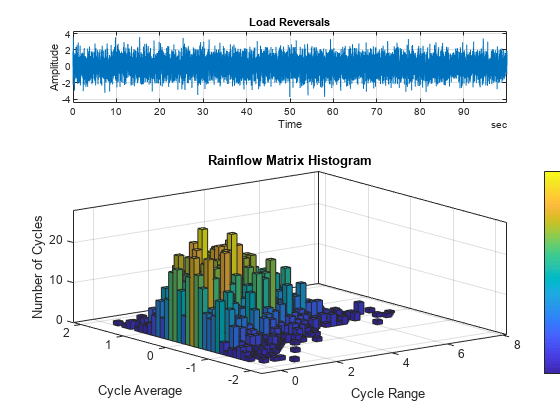
Generate a random signal sampled at 100 Hz for 100 seconds. Store the signal and its time information in a timetable.

fs = 100;
t = seconds(0:1/fs:100-1/fs)';

x = randn(size(t));
TT = timetable(t,x);

Display the reversals and the rainflow matrix of the signal.

rainflow(TT)

Cycle Counts of Identified Reversals

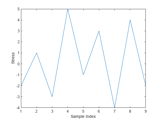
Generate a set of extrema resembling load reversals. Plot the data.

X = [-2 1 -3 5 -1 3 -4 4 -2]';

plot(X)
xlabel('Sample Index')  
ylabel('Stress')

Compute cycle counts for the data. Specify that the input consists of already identified extrema.

[C,hist,edges] = rainflow(X,'ext');

Display a histogram of cycle counts as a function of stress range.

histogram('BinEdges',edges','BinCounts',sum(hist,2))
xlabel('Stress Range')  
ylabel('Cycle Counts')

Use rainflow without output arguments to display a histogram of cycles as a function of cycle average and cycle range.

rainflow(X,'ext')

Input Arguments

x — Load time history

vector

Load time history, specified as a vector. x must have finite values.

Data Types: single | double

fs — Sample rate

positive real scalar

Sample rate, specified as a positive real scalar.

Data Types: single | double

t — Time values

vector | duration array | duration scalar

Time values, specified as a vector, a duration array, or a duration scalar representing the time interval between samples.

Example: seconds(0:1/100:1) is a duration array representing 1 second of sampling at 100 Hz.

Data Types: single | double | duration

xt — Load time history

timetable

Load time history, specified as a timetable. xt must contain increasing, finite row times. The timetable must contain only one numeric data vector with finite load values.

If a timetable has missing or duplicate time points, you can fix it using the tips in Clean Timetable with Missing, Duplicate, or Nonuniform Times.

Example: timetable(seconds(0:4)',rand(5,1)) specifies a random variable sampled at 1 Hz for 4 seconds.

Data Types: single | double

Output Arguments

c — Cycle counts

matrix

Cycle counts, returned as a matrix. c contains cycle information in its columns in this order: counts, ranges, mean values, initial sample indices, and final sample indices. See Algorithms for an example. If you specify a sample rate, a time interval, or a vector of time values, then the last two columns of c contain initial and final cycle times. If you call rainflow with a timetable as input, then the last two columns express the initial and final cycle times in seconds.

rm — Rainflow matrix

matrix

Rainflow matrix. The rows of rm correspond to cycle range, and the columns correspond to cycle mean.

rmr, rmm — Histogram bin edges

vectors

Histogram bin edges, returned as vectors. rmr and rmm contain the bin edges of the rows and columns of rm, respectively.

idx — Linear indices of reversals

vector

Linear indices of reversals, returned as a vector.

Algorithms

Fatigue analysis studies how damage accumulates in an object subjected to cyclical changes in stress. The number of cycles necessary to break the object depends on the cycle amplitude. Broadband input excitation contains cycles of diverse amplitude, and the presence of hysteresis in the object has the effect of nesting some cycles within others, either completely or partially. Rainflow counting estimates the number of load change cycles as a function of cycle amplitude.

Initially, rainflow turns the load history into a sequence of reversals. Reversals are the local minima and maxima where the load changes sign. The function counts cycles by considering a moving reference point of the sequence, Z, and a moving ordered three-point subset with these characteristics:

1. The first and second points are collectively called Y.

2. The second and third points are collectively called X.

3. In both X and Y, the points are sorted from earlier to later in time, but are not necessarily consecutive in the reversal sequence.

4. The range of X, denoted by r(X), is the absolute value of the difference between the amplitude of the first point and the amplitude of the second point. The definition of r(Y) is analogous.

The rainflow algorithm is as follows:

At the end, the function collects the different cycles and half-cycles and tabulates their ranges, their means, and the points at which they start and end. This information can then be used to produce a histogram of cycles.

Consider this reversal sequence:

Step	Z	Reversals	Three Reversals?	Y	r(Y)	X	r(X)	r(X) < r(Y)?	Z in Y?	Actions
1	A	A, B, C	Yes	AB	3	BC	4	No	Yes	Count AB as ½ cycle. Discard A. Set Z to B.
2	B	B, C	No	—	—	—	—	—	—	Read D.
3	B	B, C, D	Yes	BC	4	CD	8	No	Yes	Count BC as ½ cycle. Discard B. Set Z to C.
4	C	C, D	No	—	—	—	—	—	—	Read E.
5	C	C, D, E	Yes	CD	8	DE	6	Yes	—	Read F.
6	C	C, D, E, F	Yes	DE	6	EF	4	Yes	—	Read G.
7	C	C, D, E, F, G	Yes	EF	4	FG	7	No	No	Count EF as 1 cycle. Discard E and F.
8	C	C, D, G	Yes	CD	8	DG	9	No	Yes	Count CD as ½ cycle. Discard C. Set Z to D.
9	D	D, G	No	—	—	—	—	—	—	Read H.
10	D	D, G, H	Yes	DG	9	GH	8	Yes	—	Read J.
11	D	D, G, H, J	Yes	GH	8	HJ	7	Yes	—	Read K.
12	D	D, G, H, J, K	Yes	HJ	7	JK	4	Yes	—	Read L.
13	D	D, G, H, J, K, L	Yes	JK	4	KL	3	Yes	—	Read M.
14	D	D, G, H, J, K, L, M	Yes	KL	3	LM	5	No	No	Count KL as 1 cycle. Discard K and L.
15	D	D, G, H, J, M	Yes	HJ	7	JM	5	Yes	—	Read N.
16	D	D, G, H, J, M, N	Yes	JM	5	MN	1	Yes	—	Read P.
17	D	D, G, H, J, M, N, P	Yes	MN	1	NP	4	No	No	Count MN as 1 cycle. Discard M and N.
18	D	D, G, H, J, P	Yes	HJ	7	JP	9	No	No	Count HJ as 1 cycle. Discard H and J.
19	D	D, G, P	Yes	DG	9	GP	10	No	Yes	Count DG as ½ cycle. Discard D. Set Z to G.
20	G	G, P	Out of data	—	—	—	—	—	—	Count GP as ½ cycle.

Now collect the results.

Cycle Count	Range	Mean	Start	End
½	3	–0.5	A	B
½	4	–1	B	C
1	4	1	E	F
½	8	1	C	D
1	3	–0.5	K	L
1	1	2.5	M	N
1	7	0.5	H	J
½	9	0.5	D	G
½	10	1	G	P

Compare this to the result of running rainflow on the sequence:

q = rainflow([-2 1 -3 5 -1 3 -4 4 -3 1 -2 3 2 6])

q =

    0.5000    3.0000   -0.5000    1.0000    2.0000
    0.5000    4.0000   -1.0000    2.0000    3.0000
    1.0000    4.0000    1.0000    5.0000    6.0000
    0.5000    8.0000    1.0000    3.0000    4.0000
    1.0000    3.0000   -0.5000   10.0000   11.0000
    1.0000    1.0000    2.5000   12.0000   13.0000
    1.0000    7.0000    0.5000    8.0000    9.0000
    0.5000    9.0000    0.5000    4.0000    7.0000
    0.5000   10.0000    1.0000    7.0000   14.0000

References

[1] ASTM E1049-85(2017), "Standard Practices for Cycle Counting in Fatigue Analysis." West Conshohocken, PA: ASTM International, 2017, https://www.astm.org/e1049-85r17.html.

Extended Capabilities

C/C++ Code Generation
Generate C and C++ code using MATLAB® Coder™.

Version History

Introduced in R2017b