powerbw

Power bandwidth

Syntax

bw = powerbw(x)

bw = powerbw(x,fs)

bw = powerbw(pxx,f)

bw = powerbw(sxx,f,rbw)

bw = powerbw(___,freqlims,r)

[bw,flo,fhi,power] = powerbw(___)

powerbw(___)

Description

bw = powerbw(x) returns the 3-dB (half-power) bandwidth bw of the input signal x.

bw = powerbw(x,fs) returns the 3-dB bandwidth in terms of the sample rate fs.

bw = powerbw(pxx,f) returns the 3-dB bandwidth of the power spectral density (PSD) estimate pxx. The frequencies f correspond to the estimates in pxx.

bw = powerbw(sxx,f,rbw) computes the 3-dB bandwidth of the power spectrum estimate sxx. The frequencies f correspond to the estimates in sxx. The function uses the resolution bandwidth rbw to integrate each power estimate.

bw = powerbw(___,freqlims,r) specifies the frequency interval over which to compute the reference level. This syntax can include any combination of input arguments from previous syntaxes, as long as the second input argument is either fs or f. If the second input is passed as empty, powerbw assumes a normalized frequency. The function computes the difference in frequency between the points where the spectrum drops below the reference level by r dB or reaches an endpoint.

[bw,flo,fhi,power] = powerbw(___) also returns the lower and upper bounds of the power bandwidth and the power within those bounds.

powerbw(___) with no output arguments plots the PSD or power spectrum in the current figure window and annotates the bandwidth.

Examples

3-dB Bandwidth of Chirps

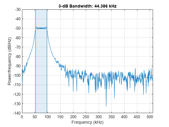
Generate 1024 samples of a chirp sampled at 1024 kHz. The chirp has an initial frequency of 50 kHz and reaches 100 kHz at the end of the sampling. Add white Gaussian noise such that the signal-to-noise ratio is 40 dB.

nSamp = 1024;
Fs = 1024e3;
SNR = 40;

t = (0:nSamp-1)'/Fs;

x = chirp(t,50e3,nSamp/Fs,100e3);
x = x + randn(size(x))*std(x)/db2mag(SNR);

Estimate the 3-dB bandwidth of the signal and annotate it on a plot of the power spectral density (PSD).

powerbw(x,Fs)

ans = 
4.4386e+04

Generate another chirp. Specify an initial frequency of 200 kHz, a final frequency of 300 kHz, and an amplitude that is twice that of the first signal. Add white Gaussian noise.

x2 = 2*chirp(t,200e3,nSamp/Fs,300e3);
x2 = x2 + randn(size(x2))*std(x2)/db2mag(SNR);

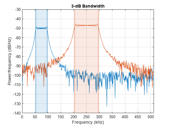
Concatenate the chirps to produce a two-channel signal. Estimate the 3-dB bandwidth of each channel.

y = powerbw([x x2],Fs)

y = 1×2
104 ×

    4.4386    9.2208

Annotate the 3-dB bandwidths of the two channels on a plot of the PSDs.

powerbw([x x2],Fs);

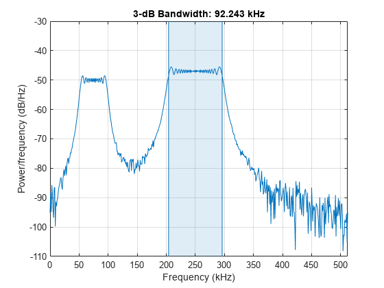
Add the two channels to form a new signal. Plot the PSD and annotate the 3-dB bandwidth.

powerbw(x+x2,Fs)

ans = 
9.2243e+04

3-dB Bandwidth of Sinusoids

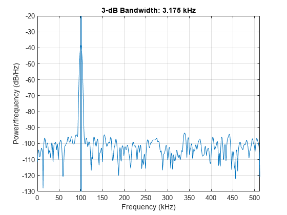
Generate 1024 samples of a 100.123 kHz sinusoid sampled at 1024 kHz. Add white Gaussian noise such that the signal-to-noise ratio is 40 dB. Reset the random number generator for reproducible results.

nSamp = 1024;
Fs = 1024e3;
SNR = 40;
rng default

t = (0:nSamp-1)'/Fs;

x = sin(2*pi*t*100.123e3);
x = x + randn(size(x))*std(x)/db2mag(SNR);

Use the periodogram function to compute the power spectral density (PSD) of the signal. Specify a Kaiser window with the same length as the signal and a shape factor of 38. Estimate the 3-dB bandwidth of the signal and annotate it on a plot of the PSD.

[Pxx,f] = periodogram(x,kaiser(nSamp,38),[],Fs);

powerbw(Pxx,f);

Generate another sinusoid, this one with a frequency of 257.321 kHz and an amplitude that is twice that of the first sinusoid. Add white Gaussian noise.

x2 = 2*sin(2*pi*t*257.321e3);
x2 = x2 + randn(size(x2))*std(x2)/db2mag(SNR);

Concatenate the sinusoids to produce a two-channel signal. Estimate the PSD of each channel and use the result to determine the 3-dB bandwidth.

[Pyy,f] = periodogram([x x2],kaiser(nSamp,38),[],Fs);

y = powerbw(Pyy,f)

y = 1×2
103 ×

    3.1753    3.3015

Annotate the 3-dB bandwidths of the two channels on a plot of the PSDs.

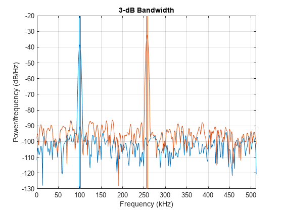
powerbw(Pyy,f);

Add the two channels to form a new signal. Estimate the PSD and annotate the 3-dB bandwidth.

[Pzz,f] = periodogram(x+x2,kaiser(nSamp,38),[],Fs);

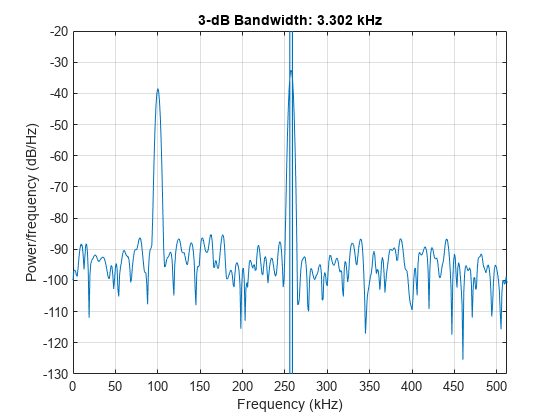
powerbw(Pzz,f);

Bandwidth of Bandlimited Signals

Generate a signal whose PSD resembles the frequency response of an 88th-order bandpass FIR filter with normalized cutoff frequencies $$0.25\pi$$ rad/sample and $$0.45\pi$$ rad/sample.

d = fir1(88,[0.25 0.45]);

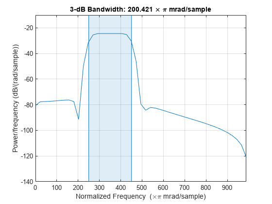
Compute the 3-dB occupied bandwidth of the signal. Specify as a reference level the average power in the band between $$0.2\pi$$ rad/sample and $$0.6\pi$$ rad/sample. Plot the PSD and annotate the bandwidth.

powerbw(d,[],[0.2 0.6]*pi,3);

Output the bandwidth, its lower and upper bounds, and the band power. Specifying a sample rate of $$2\pi$$ is equivalent to leaving the rate unset.

[bw,flo,fhi,power] = powerbw(d,2*pi,[0.2 0.6]*pi);
disp([" bw";"flo";"fhi"] + " = " + [bw;flo;fhi]/pi + "*pi")

    " bw = 0.20047*pi"
    "flo = 0.24996*pi"
    "fhi = 0.45043*pi"

fprintf('power = %.1f%% of total',power/bandpower(d)*100)

power = 96.9% of total

Add a second channel with normalized cutoff frequencies $$0.5\pi$$ rad/sample and $$0.8\pi$$ rad/sample and an amplitude that is one-tenth that of the first channel.

d = [d;fir1(88,[0.5 0.8])/10]';

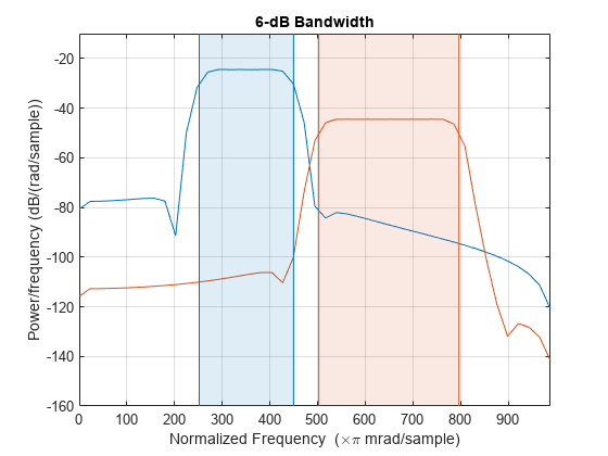
Compute the 6-dB bandwidth of the two-channel signal. Specify as a reference level the maximum power level of the spectrum.

powerbw(d,[],[],6);

Output the 6-dB bandwidth of each channel and the lower and upper bounds.

[bw,flo,fhi] = powerbw(d,[],[],6);
bds = [bw;flo;fhi];

disp([" bw";"flo";"fhi"] + " (ch_1)" + " = " + bds(:,1)/pi + "*pi")

    " bw (ch_1) = 0.19794*pi"
    "flo (ch_1) = 0.25176*pi"
    "fhi (ch_1) = 0.44971*pi"

disp([" bw";"flo";"fhi"] + " (ch_2)" + " = " + bds(:,2)/pi + "*pi")

    " bw (ch_2) = 0.29418*pi"
    "flo (ch_2) = 0.50271*pi"
    "fhi (ch_2) = 0.79689*pi"

Input Arguments

x — Input signal

vector | matrix

Input signal, specified as a vector or matrix. If x is a vector, it is treated as a single channel. If x is a matrix, then powerbw computes the power bandwidth independently for each column. x must be finite-valued.

Example: cos(pi/4*(0:159))+randn(1,160) is a single-channel row-vector signal.

Example: cos(pi./[4;2]*(0:159))'+randn(160,2) is a two-channel signal.

Data Types: single | double

fs — Sample rate

positive real scalar

Sample rate, specified as a positive real scalar. The sample rate is the number of samples per unit time. If the time is measured in seconds, then the sample rate is in hertz.

Data Types: single | double

pxx — Power spectral density

vector | matrix

Power spectral density (PSD) estimate, specified as a vector or matrix. If pxx is a one-sided estimate, then it must correspond to a real signal. If pxx is a matrix, then powerbw computes the bandwidth of each column of pxx independently.

The power spectral density must be expressed in linear units, not decibels. Use db2pow to convert decibel values to power values.

Example: [pxx,f] = periodogram(cos(pi./[4;2]*(0:159))'+randn(160,2)) specifies the periodogram PSD estimate of a noisy two-channel sinusoid sampled at 2π Hz and the frequencies at which it is computed.

Data Types: single | double

f — Frequencies

vector

Frequencies, specified as a vector. If the first element of f is 0, then powerbw assumes that the spectrum is a one-sided spectrum of a real signal. In other words, the function doubles the power value in the zero-frequency bin as it seeks the 3-dB point.

Data Types: single | double

sxx — Power spectrum estimate

vector | matrix

Power spectrum estimate, specified as a vector or matrix. If sxx is a matrix, then powerbw computes the bandwidth of each column of sxx independently.

The power spectrum must be expressed in linear units, not decibels. Use db2pow to convert decibel values to power values.

Example: [sxx,w] = periodogram(cos(pi./[4;2]*(0:159))'+randn(160,2),"power") specifies the periodogram power spectrum estimate of a two-channel sinusoid embedded in white Gaussian noise and the normalized frequencies at which it is computed.

Data Types: single | double

rbw — Resolution bandwidth

positive scalar

Resolution bandwidth, specified as a positive scalar. The resolution bandwidth is the product of two values: the frequency resolution of the discrete Fourier transform and the equivalent noise bandwidth of the window used to compute the PSD.

Data Types: single | double

freqlims — Frequency limits

two-element vector

Frequency limits, specified as a two-element vector of real values. If you specify freqlims, then the reference level is the average power level in the reference band. If you do not specify freqlims, then the reference level is the maximum power level of the spectrum. freqlims must lie within the target band.

Data Types: single | double

r — Power level drop

10*log10(2) (default) | positive real scalar

Power level drop, specified as a positive real scalar expressed in dB.

Data Types: single | double

Output Arguments

bw — Power bandwidth

scalar | vector

Power bandwidth, returned as a scalar or vector.

• If you specify a sample rate, then bw has the same units as fs.

• If you do not specify a sample rate, then bw has units of rad/sample.

flo, fhi — Bandwidth frequency bounds

scalars | vectors

Bandwidth frequency bounds, returned as scalars.

power — Power stored in bandwidth

scalar | vector

Power stored in bandwidth, returned as a scalar or vector.

Algorithms

To determine the 3-dB bandwidth, powerbw computes a periodogram power spectrum estimate using a rectangular window and takes the maximum of the estimate as a reference level. The bandwidth is the difference in frequency between the points where the spectrum drops at least 3 dB below the reference level. If the signal reaches one of its endpoints before dropping by 3 dB, then powerbw uses the endpoint to compute the difference.

Extended Capabilities

C/C++ Code Generation
Generate C and C++ code using MATLAB® Coder™.

GPU Arrays

Accelerate code by running on a graphics processing unit (GPU) using Parallel Computing Toolbox™.

This function fully supports GPU arrays. For more information, see Run MATLAB Functions on a GPU (Parallel Computing Toolbox).

Version History

Introduced in R2015a

R2023a: Use gpuArray objects

The powerbw function supports gpuArray objects. You must have Parallel Computing Toolbox™ to use this functionality.