Main Content

instfreq

Estimate instantaneous frequency

Description

example

ifq = instfreq(x,fs) estimates the instantaneous frequency of a signal, x, sampled at a rate fs. If x is a matrix, then the function estimates the instantaneous frequency independently for each column and returns the result in the corresponding column of ifq.

example

ifq = instfreq(x,t) estimates the instantaneous frequency of x sampled at the time values stored in t.

example

ifq = instfreq(xt) estimates the instantaneous frequency of a signal stored in the MATLAB® timetable xt. The function treats all variables in the timetable and all columns inside each variable independently.

example

ifq = instfreq(tfd,fd,td) estimates the instantaneous frequency of the signal whose time-frequency distribution, tfd, is sampled at the frequency values stored in fd and the time values stored in td.

example

ifq = instfreq(___,Name=Value) specifies additional options for any of the previous syntaxes using name-value arguments. You can specify the algorithm used to estimate the instantaneous frequency or the frequency limits used in the computation.

example

[ifq,t] = instfreq(___) also returns t, a vector of sample times corresponding to ifq.

example

instfreq(___) with no output arguments plots the estimated instantaneous frequency.

Examples

collapse all

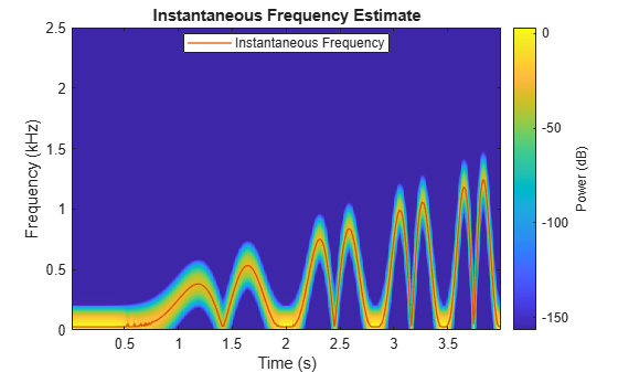
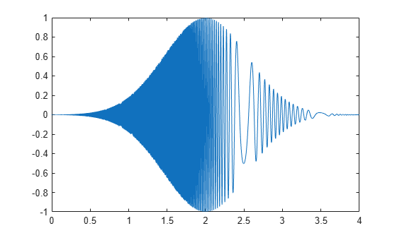
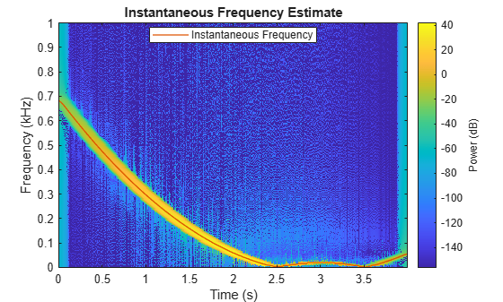
Generate a signal sampled at 5 kHz for 4 seconds. The signal consists of a set of pulses of decreasing duration separated by regions of oscillating amplitude and fluctuating frequency with an increasing trend. Plot the signal.

fs = 5000;
t = 0:1/fs:4-1/fs;

s = besselj(0,1000*(sin(2*pi*t.^2/8).^4));

% To hear, type sound(s,fs)

plot(t,s)

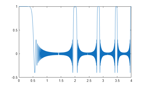
Estimate the time-dependent frequency of the signal as the first moment of the power spectrogram. Plot the power spectrogram and overlay the instantaneous frequency.

instfreq(s,fs)

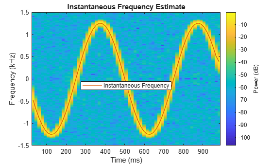
Generate a complex-valued signal that consists of a chirp with sinusoidally varying frequency content. The signal is sampled at 3 kHz for 1 second and is embedded in white Gaussian noise.

fs = 3000;
t = 0:1/fs:1-1/fs;
x = exp(2j*pi*100*cos(2*pi*2*t))+randn(size(t))/100;

Estimate the time-dependent frequency of the signal as the first moment of the power spectrogram. This is the only method that instfreq supports for complex-valued signals. Plot the power spectrogram and overlay the instantaneous frequency.

instfreq(x,t)

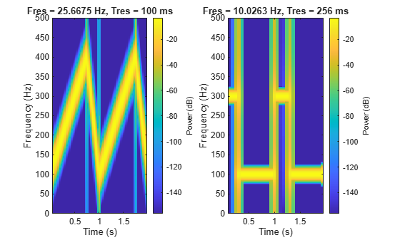
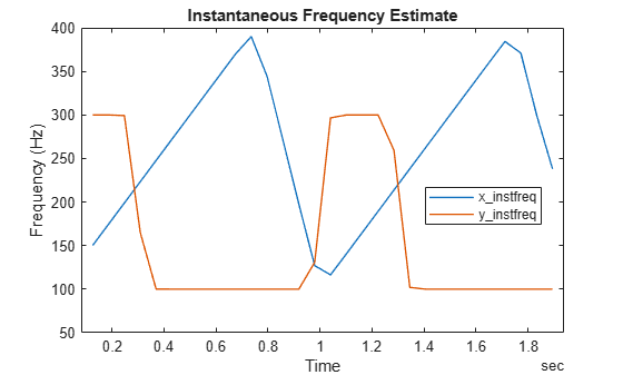
Create a two-channel signal, sampled at 1 kHz for 2 seconds, consisting of two voltage-controlled oscillators.

  • In one channel, the instantaneous frequency varies with time as a sawtooth wave whose maximum is at 75% of the period.

  • In the other channel, the instantaneous frequency varies with time as a square wave with a duty cycle of 30%.

Plot the spectrograms of the two channels. Specify a time resolution of 0.1 second for the sawtooth channel and a frequency resolution of 10 Hz for the square channel.

fs = 1000;
t = (0:1/fs:2)';
x = vco(sawtooth(2*pi*t,0.75),[0.1 0.4]*fs,fs);
y = vco(square(2*pi*t,30),[0.1 0.3]*fs,fs);

subplot(1,2,1)
pspectrum(x,fs,'spectrogram','TimeResolution',0.1)
subplot(1,2,2)
pspectrum(y,fs,'spectrogram','FrequencyResolution',10)

Store the signal in a timetable. Compute and display the instantaneous frequency.

xt = timetable(seconds(t),x,y);

clf
instfreq(xt)

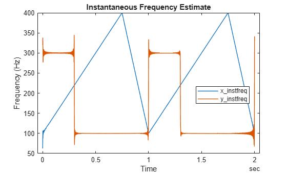
Repeat the computation using the analytic signal.

instfreq(xt,'Method','hilbert')

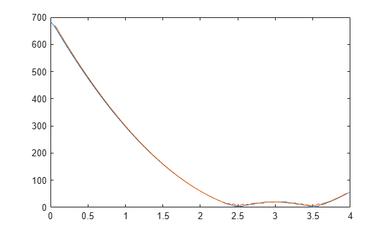
Generate a quadratic chirp modulated by a Gaussian. Specify a sample rate of 2 kHz and a signal duration of 4 seconds.

fs = 2000;
t = 0:1/fs:4-1/fs;

q = chirp(t-1,0,1/2,20,'quadratic',100,'convex').*exp(-1.7*(t-2).^2);
plot(t,q)

Use the pspectrum function with default settings to estimate the power spectrum of the signal. Use the estimate to compute the instantaneous frequency.

[p,f,t] = pspectrum(q,fs,'spectrogram');

instfreq(p,f,t)

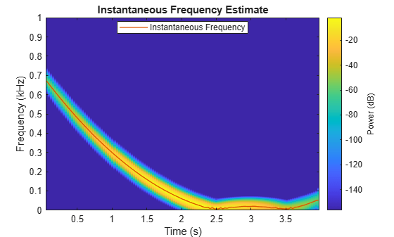
Repeat the calculation using the synchrosqueezed Fourier transform. Use a 500-sample Hann window to divide the signal into segments and window them.

[s,sf,st] = fsst(q,fs,hann(500));

instfreq(abs(s).^2,sf,st)

Compare the instantaneous frequencies found using the two different methods.

[psf,pst] = instfreq(p,f,t);
[fsf,fst] = instfreq(abs(s).^2,sf,st);

plot(fst,fsf,pst,psf)

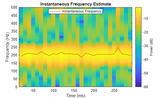
Generate a sinusoidal signal sampled at 1 kHz for 0.3 second and embedded in white Gaussian noise of variance 1/16. Specify a sinusoid frequency of 200 Hz. Estimate and display the instantaneous frequency of the signal.

fs = 1000;
t = (0:1/fs:0.3-1/fs)';

x = sin(2*pi*200*t) + randn(size(t))/4;

instfreq(x,t)

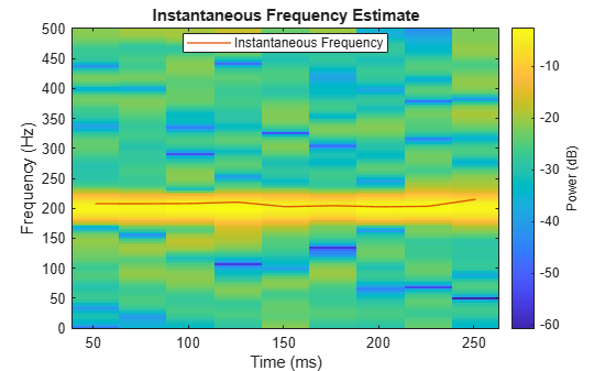
Estimate the instantaneous frequency of the signal again, but now use a time-frequency distribution with a coarse frequency resolution of 25 Hz as input.

[p,fd,td] = pspectrum(x,t,'spectrogram','FrequencyResolution',25);

instfreq(p,fd,td)

Generate a signal that consists of a chirp whose frequency varies sinusoidally between 300 Hz and 1200 Hz. The signal is sampled at 3 kHz for 2 seconds.

fs = 3e3;
t = 0:1/fs:2;
y = chirp(t,100,1,200,"quadratic");
y = vco(cos(2*pi*t),[0.1 0.4]*fs,fs);

Use instfreq to compute the instantaneous frequency of the signal and the corresponding sample times. Verify that the output corresponds to the noncentralized first-order conditional spectral moment of the time-frequency distribution of the signal as computed by tfsmoment (Predictive Maintenance Toolbox).

[z,tz] = instfreq(y,fs);
[a,ta] = tfsmoment(y,fs,1,Centralize=false);

plot(tz,z,ta,a,".")
legend("instfreq","tfsmoment")

Use instbw to compute the instantaneous bandwidth of the signal and the corresponding sample times. Specify a scale factor of 1. Verify that the output corresponds to the square root of the centralized second-order conditional spectral moment of the time-distribution of the signal. In other words, instbw generates a standard deviation and tfsmoment generates a variance.

[w,tw] = instbw(y,fs,ScaleFactor=1);
[m,tm] = tfsmoment(y,fs,2);

plot(tw,w,tm,sqrt(m),".")
legend("instbw","tfsmoment")

Input Arguments

collapse all

Input signal, specified as a vector or matrix. If x is a vector, then instfreq treats it as a single channel. If x is a matrix, then the function computes the instantaneous frequency independently for each column and returns the result in the corresponding column of ifq.

Example: sin(2*pi*(0:127)/16)+randn(1,128)/100 specifies a noisy sinusoid

Example: [2 1].*sin(2*pi*(0:127)'./[16 64]) specifies a two-channel sinusoid.

Data Types: single | double
Complex Number Support: Yes

Sample rate, specified as a positive scalar. The sample rate is the number of samples per unit time. If the unit of time is seconds, then the sample rate is in Hz.

Data Types: single | double | int8 | int16 | int32 | int64 | uint8 | uint16 | uint32 | uint64

Sample times, specified as a real vector, a duration scalar, a duration array, or a datetime array.

  • duration scalar — The time interval between consecutive samples of x.

  • Real vector, duration array, or datetime array — The time instant corresponding to each element of x.

Example: seconds(1) specifies a 1-second lapse between consecutive measurements of a signal.

Example: seconds(0:8) specifies that a signal is sampled at 1 Hz for 8 seconds.

Data Types: single | double | duration | datetime

Input timetable. xt must contain increasing, finite row times.

If a timetable has missing or duplicate time points, you can fix it using the tips in Clean Timetable with Missing, Duplicate, or Nonuniform Times.

Example: timetable(seconds(0:4)',randn(5,1)) specifies a random process sampled at 1 Hz for 4 seconds.

Example: timetable(seconds(0:4)',randn(5,3),randn(5,4)) contains a three-channel random process and a four-channel random process, both sampled at 1 Hz for 4 seconds.

Data Types: single | double
Complex Number Support: Yes

Time-frequency distribution, specified as a matrix sampled at the frequencies stored in fd and the time values stored in td. This input argument is supported only when Method is set to "tfmoment".

Example: [p,f,t] = pspectrum(sin(2*pi*(0:511)/4),4,"spectrogram") specifies the time-frequency distribution of a 1 Hz sinusoid sampled at 4 Hz for 128 seconds, and also the frequencies and times at which it is computed.

Data Types: single | double

Frequency and time values for time-frequency distribution, specified as vectors. These input arguments are supported only when Method is set to "tfmoment".

Example: [p,f,t] = pspectrum(sin(2*pi*(0:511)/4),4,"spectrogram") specifies the time-frequency distribution of a 1 Hz sinusoid sampled at 4 Hz for 128 seconds, and also the frequencies and times at which it is computed.

Data Types: single | double

Name-Value Arguments

Specify optional pairs of arguments as Name1=Value1,...,NameN=ValueN, where Name is the argument name and Value is the corresponding value. Name-value arguments must appear after other arguments, but the order of the pairs does not matter.

Before R2021a, use commas to separate each name and value, and enclose Name in quotes.

Example: 'Method','tfmoment','FrequencyLimits',[25 50] computes the instantaneous frequency of the input in the range from 25 Hz to 50 Hz by finding the first conditional spectral moment of the time-frequency distribution.

Frequency range, specified as a two-element vector in Hz. If you do not specify FrequencyLimits, then this argument defaults to [0 fs/2] for real-valued signals and to [-fs/2 fs/2] for complex-valued signals. This argument is supported only when Method is set to "tfmoment".

Data Types: single | double

Computation method, specified as either "tfmoment" or "hilbert".

  • "tfmoment" — Compute the instantaneous frequency as the first conditional spectral moment of the time-frequency distribution of x. If x is nonuniformly sampled, then the function interpolates the signal to a uniform grid to compute instantaneous frequencies.

  • "hilbert" — Compute the instantaneous frequency as the derivative of the phase of the analytic signal of x found using the Hilbert transform. This method accepts only uniformly sampled, real-valued signals and does not support time-frequency distribution input.

Output Arguments

collapse all

Instantaneous frequency, returned as a vector, a matrix, or a timetable with the same dimensions as the input.

Data Types: single | double

Times of frequency estimates, returned as a real vector, a duration array, or a datetime array.

Data Types: single | double

Note

If t, fd, or td are in single precision and the input vector or matrix is in double precision, then the function returns the output in single precision. The output data type does not depend on the sample rate data type.

More About

collapse all

Instantaneous Frequency

The instantaneous frequency of a nonstationary signal is a time-varying parameter that relates to the average of the frequencies present in the signal as it evolves [1], [2].

  • If 'Method' is set to 'tfmoment', then instfreq estimates the instantaneous frequency as the first conditional spectral moment of the time-frequency distribution of the input signal. The function:

    1. Computes the spectrogram power spectrum P(t,f) of the input using the pspectrum function and uses the spectrum as a time-frequency distribution.

    2. Estimates the instantaneous frequency using

      finst(t)=0fP(t,f)df0P(t,f)df.

  • If 'Method' is set to 'hilbert', then instfreq estimates the instantaneous frequency as the derivative of the phase of the analytic signal of the input. The function:

    1. Computes the analytic signal, xA, of the input using the hilbert function.

    2. Estimates the instantaneous frequency using

      finst(t)=12πdϕdt,

      where ϕ is the phase of the analytic signal of the input.

References

[1] Boashash, Boualem. “Estimating and Interpreting the Instantaneous Frequency of a Signal. I. Fundamentals.” Proceedings of the IEEE® 80, no. 4 (April 1992): 520–538. https://doi.org/10.1109/5.135376.

[2] Boashash, Boualem. "Estimating and Interpreting The Instantaneous Frequency of a Signal. II. Algorithms and Applications." Proceedings of the IEEE 80, no. 4 (May 1992): 540–568. https://doi.org/10.1109/5.135378.

Extended Capabilities

C/C++ Code Generation
Generate C and C++ code using MATLAB® Coder™.

Version History

Introduced in R2018a

expand all

See Also

| | | (Predictive Maintenance Toolbox) | (Predictive Maintenance Toolbox) | (Predictive Maintenance Toolbox)