Main Content

serdes.DFECDR

Decision feedback equalizer (DFE) with clock and data recovery (CDR)

Description

The serdes.DFECDR System object™ adaptively processes a sample-by-sample input signal or analytically processes an impulse response vector input signal to remove distortions at post-cursor taps.

The DFE modifies baseband signals to minimize the intersymbol interference (ISI) at the clock sampling times. The DFE samples data at each clock sample time and adjusts the amplitude of the waveform by a correction voltage.

For impulse response processing, the hula-hoop algorithm is used to find the clock sampling locations. The zero-forcing algorithm is then used to determine the N correction factors necessary to have no ISI at the N subsequent sampling locations, where N is the number of DFE taps.

For sample-by-sample processing, the clock recovery is accomplished by a first order phase tracking model. The bang-bang phase detector utilizes the unequalized edge samples and equalized data samples to determine the optimum sampling location. The DFE correction voltage for the N-th tap is adaptively found by finding a voltage that compensates for any correlation between two data samples spaced by N symbol times. This requires a data pattern that is uncorrelated with the channel ISI for correct adaptive behavior.

To equalize the input signal:

  1. Create the serdes.DFECDR object and set its properties.

  2. Call the object with arguments, as if it were a function.

To learn more about how System objects work, see What Are System Objects?

Creation

Description

dfecdr = serdes.DFECDR returns a DFECDR object that modifies an input waveform with the DFE and determines the clock sampling times. The system object estimates the data symbol according to the Bang-Bang CDR algorithm.

dfecdr = serdes.DFECDR(Name,Value) sets properties using one or more name-value pairs. Enclose each property name in quotes. Unspecified properties have default values.

Example: dfecdr = serdes.DFECDR('Mode',1) returns a DFECDR object that applies specified DFE tap weights to input waveform.

Properties

expand all

Unless otherwise indicated, properties are nontunable, which means you cannot change their values after calling the object. Objects lock when you call them, and the release function unlocks them.

If a property is tunable, you can change its value at any time.

For more information on changing property values, see System Design in MATLAB Using System Objects.

DFE Properties

DFE operating mode, specified as 0, 1, or 2. The operating mode you select determines the DFE tap weights values that the object applies to the input waveform.

Mode ValueDFE ModeDFE Operation
0OffThe object bypasses DFE and the input waveform remains unchanged.
1FixedThe object applies the DFE tap weights specified in TapWeights to the input waveform.
2AdaptThe object determines the optimum DFE tap weights and applies them to the input waveform.

Data Types: double

Initial DFE tap weights, specified as a row vector in volts. The length of the vector determines the number of taps. The vector elements signify the tap weights or tap strength. Set the tap weight to zero to initialize the tap.

Data Types: double

Minimum value of the adapted tap weights, specified as a real scalar or a real-valued row vector in volts. Specify as a scalar to apply to apply the same minimum value to all the DFE taps, or specify as a vector that has the same length as the TapWeights.

Data Types: double

Maximum value of the adapted tap weights, specified as a nonnegative real scalar or a nonnegative real-valued row vector in volts. Specify as a scalar to apply the same maximum value to all the DFE taps, or specify as a vector that has the same length as the TapWeights.

Data Types: double

Controls for update rate of tap weights, specified as a unitless nonnegative real scalar. Increase the value of this property for the DFE adaptation to converge faster at the expense of more noise in the DFE tap values.

Data Types: double

DFE adaptive step resolution, specified as a nonnegative real scalar or a nonnegative real-valued row vector in volts. Specify as a scalar to apply the same value to all the DFE taps, or specify as a vector that has the same length as TapWeights.

EqualizationStep specifies the minimum change in DFE taps from one time step to the next to mimic hardware limitations. Setting EqualizationStep to zero yields DFE tap values without any resolution limitation.

Data Types: double

Multiply DFE tap weights by a factor of two, specified as true or false. Set this property to true to multiply the DFE tap weights by a factor of two.

The output of the slicer in the serdes.DFECDR System object from the SerDes Toolbox™ is [-0.5 0.5]. But some industry applications require the slicer output to be [-1 1]. Taps2x allows you to quickly double the DFE tap weights to change the slicer reference.

CDR Properties

Determine the CDR order to enable phase and frequency tracking.

  • 1st order — Only tracks the phase.

  • 2nd order — Tracks both the phase and frequency.

Early or late CDR count threshold to trigger a phase update, specified as a unitless real positive integer greater than 4. Increasing the value of Count provides a more stable output clock phase at the expense of convergence speed. Because the bit decisions are made at the clock phase output, a more stable clock phase has a better bit error rate (BER).

Count also controls the bandwidth of the CDR which is approximately calculated by using the equation:

Bandwidth=1Symbol time · Early/late threshold count · Step

Data Types: double

Clock phase resolution, specified as a real scalar in fraction of symbol time. ClockStep is the inverse of the number of phase adjustments in CDR.

Data Types: double

Clock phase offset, specified as a real scalar in the range [−0.5, 0.5] in fraction of symbol time. PhaseOffset is used to manually shift the clock probability distribution function (PDF) for better BER.

Data Types: double

Reference clock offset impairment, specified as a real scalar in the range [−300, 300] in parts per million (ppm). ReferenceOffset is the deviation between transmitter oscillator frequency and receiver oscillator frequency.

Data Types: double

Sampling latch metastability voltage, specified as a real scalar in volts (V). If the data sample voltage lies within the region (±Sensitivity), there is a 50% probability of bit error.

Data Types: double

Clock phase detector option used in the clock data recovery. You can choose between bang-bang (Alexander) or baud-rate type-A (Mueller-Muller).

Internal gain for the frequency tracking loop, specified as a nonnegative real scalar.

Data Types: double

Once every FrequencyCount symbols, update the system phase rotator clock with the frequency estimate.

Data Types: double

Advanced Properties

Time of a single symbol duration, specified as a real scalar in seconds (s).

Data Types: double

Uniform time step of the waveform, specified as a real scalar in seconds (s).

Data Types: double

Modulation scheme, specified as 2, 3 or 4.

Modulation ValueModulation Scheme
2Non-return to zero (NRZ)
3Three-level pulse amplitude modulation (PAM3)
4Four-level pulse amplitude modulation (PAM4)

Note

IBIS does not support a PAM3 modulation scheme, so you cannot export the System object to IBIS-AMI model if you set the modulation scheme to PAM3.

Data Types: double

Input waveform type, specified as one of these:

  • 'Sample' — A sample-by-sample input signal.

  • 'Impulse' — An impulse-response input signal.

Data Types: char

Usage

Description

y = dfecdr(x)

Input Arguments

expand all

Input baseband signal, specified as a scalar or vector. If you set the WaveType property to 'Sample', then the input signal is a sample-by-sample signal specified as a scalar. If you set the WaveType property to 'Impulse', the input signal is an impulse-response vector signal.

Output Arguments

expand all

Estimated channel output. If the input signal is a sample-by-sample signal specified as a scalar, then the output is also scalar. If the input signal is an impulse response vector signal, the output is also a vector.

Estimated DFE tap weight values, returned as a vector.

Relative recovered clock phase, returned as a units of SymbolTime in the range [0,1].

AMI clock bus, returned as a structure.

FieldDescription
clockTimeTime taken to sample the data signal.
clockValidOnRisingValid clock time value on the rising edge of a signal.

Bus containing additional interior CDR signals, returned as a structure.

FieldDescription
clockPhaseRelative clock phase in units of SymbolTime in the range of [0,1].
symbolRecoveredSymbol recovered from data signal at ClockTime.
voltageSampleVoltage observed from the data signal at ClockTime.
PAM4ThresholdThe estimated upper eye at PAM4 threshold.
CDRedgeVoltageThe voltage observed from the data signal at ClockTimeSymbolTime/2.
CDRCounterThe bang-bang CDR internal counter used to trigger samples.
CDREarlyLateCountThe bang-bang CDR accumulated (or filtered) signal used to trigger updated to the CDR phase.
PAMSymbolMiddleVoltageEstimated PAM4 symbol voltage of the inner eye outer envelope to estimate PAM threshold.
PAMSymbolOuterVoltageEstimated PAM4 outer envelope voltage to estimate PAM threshold.
EyeHeightAbsAveEstimates eye height.
PAMThresholdArray of PAM thresholds for each eye in the PAMn modulation. If the modulation scheme is PAMn, the first (n-1) eyes contain the valid thresholds. The rest of the entries are zero-padded.
PhaseErrorPhase detector error.
FreqEstimateFrequency estimate for the 2nd order or frequency tracking loop.

Object Functions

To use an object function, specify the System object as the first input argument. For example, to release system resources of a System object named obj, use this syntax:

release(obj)

expand all

stepRun System object algorithm
releaseRelease resources and allow changes to System object property values and input characteristics
resetReset internal states of System object

Examples

collapse all

This example shows how to process impulse response of a channel using serdes.DFECDR System object™.

Use a symbol time of 100 ps. There are 16 samples per symbol. The channel has 14 dB loss.

SymbolTime = 100e-12;         
SamplesPerSymbol = 16;
dbloss = 14;                  
NumberOfDFETaps = 2;

Calculate the sample interval.

dt = SymbolTime/SamplesPerSymbol; 

Create the DFECDR object. The object adaptively applies optimum DFE tap weights to input impulse response.

DFE1 = serdes.DFECDR('SymbolTime',SymbolTime,'SampleInterval',dt,...
      'Mode',2,'WaveType','Impulse','TapWeights',zeros(NumberOfDFETaps,1));

Create the channel impulse response.

channel = serdes.ChannelLoss('Loss',dbloss,'dt',dt,...
      'TargetFrequency',1/SymbolTime/2);
impulseIn = channel.impulse;

Process the impulse response with DFE.

[impulseOut,TapWeights] = DFE1(impulseIn);

Convert the impulse response to a pulse, a waveform and an eye diagram for visualization.

ord = 6;
dataPattern = prbs(ord,2^ord-1)-0.5;

pulseIn = impulse2pulse(impulseIn,SamplesPerSymbol,dt);
waveIn = pulse2wave(pulseIn,dataPattern,SamplesPerSymbol);
eyeIn = reshape(waveIn,SamplesPerSymbol,[]);

pulseOut = impulse2pulse(impulseOut,SamplesPerSymbol,dt);
waveOut = pulse2wave(pulseOut,dataPattern,SamplesPerSymbol);
eyeOut = reshape(waveOut,SamplesPerSymbol,[]);

Create the time vectors.

t = dt*(0:length(pulseOut)-1)/SymbolTime;
teye = t(1:SamplesPerSymbol);
t2 = dt*(0:length(waveOut)-1)/SymbolTime;

Plot the resulting waveforms.

figure
plot(t,pulseIn,t,pulseOut)
legend('Input','Output')
title('Pulse Response Comparison')
xlabel('SymbolTimes'),ylabel('Voltage')
grid on
axis([41 55 -0.1 0.4])  

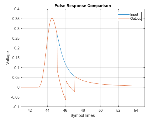
figure
plot(t2,waveIn,t2,waveOut)
legend('Input','Output')
title('Waveform Comparison')
xlabel('SymbolTimes'),ylabel('Voltage')
grid on 

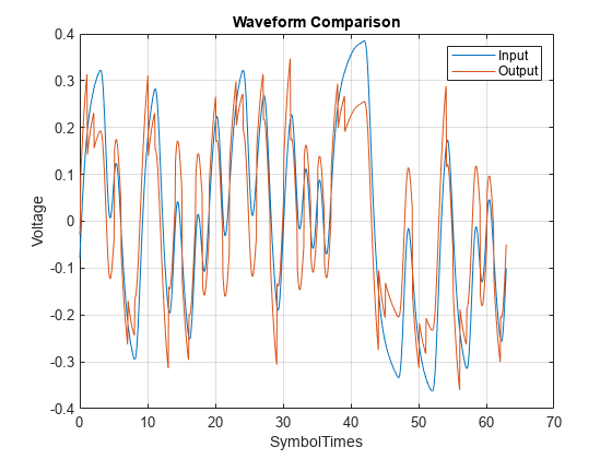
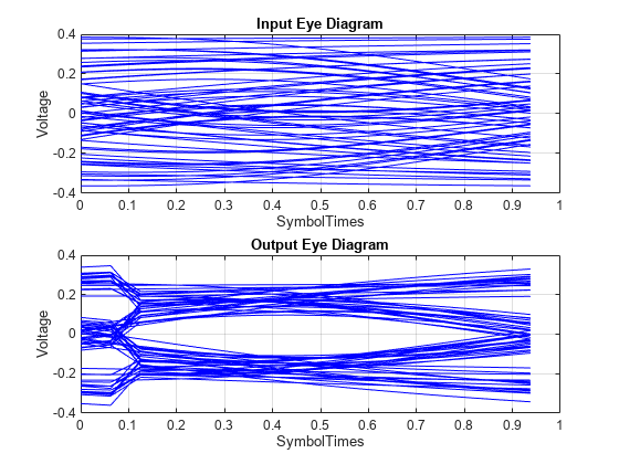
figure
subplot(211),plot(teye,eyeIn,'b')
xlabel('SymbolTimes'),ylabel('Voltage')
grid on
title('Input Eye Diagram')
subplot(212),plot(teye,eyeOut,'b')
xlabel('SymbolTimes'),ylabel('Voltage')
grid on
title('Output Eye Diagram')

This example shows how to process impulse response of a channel one sample at a time using serdes.DFECDR System object™.

Use a symbol time of 100 ps, with 8 samples per symbol. The channel loss is 14 dB. Select 12-th order pseudorandom binary sequence (PRBS), and simulate the first 20000 symbols.

SymbolTime = 100e-12;           
SamplesPerSymbol = 8;
dbloss = 14;                    
NumberOfDFETaps = 2;
prbsOrder = 12;                 
M = 20000;                      

Calculate the sample interval.

dt = SymbolTime/SamplesPerSymbol;

Create the DFECDR System object. Process the channel one sample at a time by setting the input waveforms to 'sample' type. The object adaptively applies the optimum DFE tap weights to input waveform.

DFE2 = serdes.DFECDR('SymbolTime',SymbolTime,'SampleInterval',dt,...
      'Mode',2,'WaveType','Sample','TapWeights',zeros(NumberOfDFETaps,1),...
      'EqualizationStep',0,'EqualizationGain',1e-3);

Create the channel impulse response.

channel = serdes.ChannelLoss('Loss',dbloss,'dt',dt,...
      'TargetFrequency',1/SymbolTime/2);

Initialize the PRBS generator.

[dataBit,prbsSeed]=prbs(prbsOrder,1);

Generate the sample-by-sample eye diagram.

%Loop through one symbol at a time.
inSymbol = zeros(SamplesPerSymbol,1);
outWave = zeros(SamplesPerSymbol*M,1);
dfeTapWeightHistory = nan(M,NumberOfDFETaps);

for ii = 1:M
  %Get new symbol
      [dataBit,prbsSeed]=prbs(prbsOrder,1,prbsSeed);    
      inSymbol(1:SamplesPerSymbol) = dataBit-0.5;
      
   %Convolve input waveform with channel
      y = channel(inSymbol);
      
   %Process one sample at a time through the DFE
      for jj = 1:SamplesPerSymbol
          [outWave((ii-1)*SamplesPerSymbol+jj),TapWeights] = DFE2(y(jj));
      end
      
    %Save DFE taps
      dfeTapWeightHistory(ii,:) = TapWeights; 
end

Plot the DFE adaptation history.

figure
plot(dfeTapWeightHistory)
grid on
legend('TapWeights(1)','TapWeights(2)')
xlabel('Symbols')
ylabel('Voltage')
title('DFE Taps')   

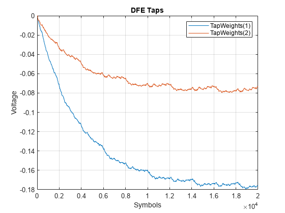
You can observe from the plot that the DFE adaptation is approximately complete after the first 10000 symbols, so these can be truncated from the array. Then plot the eye diagram by applying the reshape function to the array of symbols.

foldedEye = reshape(outWave(10000*SamplesPerSymbol+1:M*SamplesPerSymbol),SamplesPerSymbol,[]);
t = dt*(0:SamplesPerSymbol-1);
figure,plot(t,foldedEye,'b');
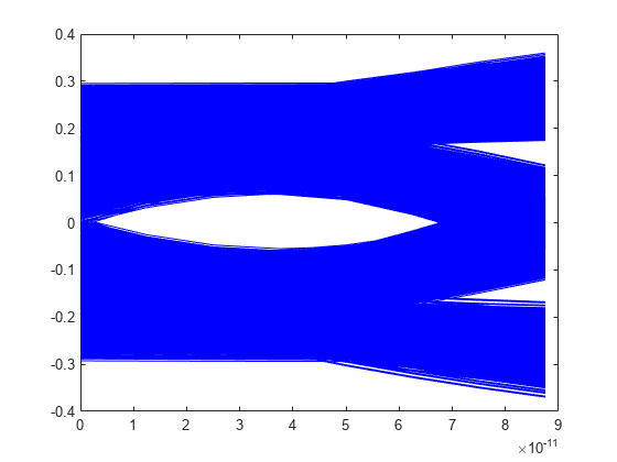
More About

expand all

Extended Capabilities

Version History

Introduced in R2019a