Model NR NTN Channel

R2026b

This example uses:

This example shows how to model these New Radio (NR) non-terrestrial network (NTN) channels.

Flat fading channel, as defined in 3GPP TR 38.811 section 6.7.1 [1]
Frequency selective fading clustered delay line (CDL) channel, as defined in 3GPP TR 38.811 section 6.9.1 [1]
Frequency selective fading tapped delay line (TDL) channel, as defined in 3GPP TR 38.811 section 6.9.2 [1]

These channels model different NTN deployment scenarios, covering both geosynchronous orbit (GSO) satellites and non-geosynchronous orbit (NGSO) satellites.

Introduction

In this example, you generate the path gains of the NTN channel model by applying the Doppler shift due to satellite movement, to the path gains generated from a base channel model. The example implements the base channel model for each NTN channel model using these standards:

Flat fading narrowband channel — ITU-R P.681-11, which defines the propagation data for a land mobile-satellite (LMS) channel [4].
Frequency selective CDL channel — 3GPP TR 38.901 section 6.9.1, which defines the terrestrial CDL channel [2].
Frequency selective TDL channel — 3GPP TR 38.901 section 6.9.2, which defines the terrestrial TDL channel [2].

The Doppler shift due to satellite movement depends on the satellite orbit, elevation angle, and carrier frequency. The Doppler shift due to satellite motion $f_{d, sat}$ , as defined in 3GPP TR 38.811 section 6.7.1 and section 6.9.2 [1], is:

$f_{d, sat} = (\frac{ν_{sat}}{c}) * (\frac{R}{R + h} \cos (α_{model})) * f_{c}$

$c$ is the speed of light ( $299792458 \frac{m}{s}$ ).
$R$ is the earth radius ( $6371000 m$ ).
$h$ is the satellite altitude.
$α_{model}$ is the satellite elevation angle.
$f_{c}$ is the carrier frequency.
$ν_{sat}$ is the satellite speed and is given by $\sqrt{\frac{GM}{(R + h)}}$ , where G is gravitational constant ( $6.6743 * 10^{- 11} \frac{m^{3}}{kg s^{2}}$ ) and M is mass of Earth ( $5.9722 * 10^{24} kg$ ).

This example uses:

dopplerShiftCircularOrbit function to calculate the Doppler shift due to satellite movement
p681LMSChannel System object™ to model the NTN narrowband channel
nrCDLChannel (5G Toolbox) System object™ to model the NTN CDL channel
nrTDLChannel (5G Toolbox) System object™ to model the NTN TDL channel

Set NTN Channel Common Parameters

Set the common parameters required to model an NTN channel. This example models a low Earth orbit (LEO) satellite moving at an altitude of 600 km and is operating in the S-band. Assume a mobile or user equipment (UE) speed of 3 km/hr. These default parameters are from 3GPP TR 38.821 table 6.1.2-4 [3].

commonParams = struct;
commonParams.CarrierFrequency = 2e9;              % In Hz
commonParams.ElevationAngle = 50;                 % In degrees
commonParams.SatelliteAltitude = 600000;          % In m
commonParams.MobileAltitude = 0;                  % In m
commonParams.MobileSpeed = 3*1000/3600;           % In m/s
% Set the random stream and seed, for reproducibility
commonParams.RandomStream = "mt19937ar with seed";
commonParams.Seed = 73;
% Set the number of sinusoids used in generation of Doppler spread
commonParams.NumSinusoids = 48;
% Calculate the Doppler shift due to satellite movement
satelliteDopplerShift = dopplerShiftCircularOrbit(...
    commonParams.ElevationAngle,commonParams.SatelliteAltitude,...
    commonParams.MobileAltitude,commonParams.CarrierFrequency);
% Calculate the maximum Doppler shift due to mobile movement
c = physconst("lightspeed");
mobileMaxDoppler = commonParams.MobileSpeed*commonParams.CarrierFrequency/c;

Generate and Assign Channel Input Signals

This example generates two transmit waveforms, a narrowband Digital Video Broadcasting Satellite Second Generation extended (DVB-S2X) waveform and a wideband 5G downlink waveform.

You can select the input waveform independently for each NTN channel. By default:

The NTN narrowband channel uses the DVB-S2X waveform because its narrow bandwidth is well suited to evaluating flat-fading channel behavior.
The NTN CDL and NTN TDL channels use the wideband 5G waveform because frequency-selective fading is only visible when the signal bandwidth is comparable to the channel coherence bandwidth.

rng(commonParams.Seed)

% Generate a narrowband DVB-S2X signal
s2xWaveGen = dvbs2xWaveformGenerator;
numFrames = 3;
syncBits = [0 1 0 0 0 1 1 1]';                              % Sync byte for a TS packet (47 hex)
pktLen = 1496;                                              % User packet length without sync bits
numPkts = s2xWaveGen.MinNumPackets*numFrames;
txPkts = [repmat(syncBits,1,numPkts); ...
    randi([0 1],pktLen,numPkts)];
dvbs2xSignal = s2xWaveGen(txPkts(:));
symbolRate = 1e6;                                           % In symbols/s
dvbs2xSampleRate = symbolRate*s2xWaveGen.SamplesPerSymbol;  % In Hz

% Generate a 5G downlink signal with 50 MHz bandwidth and 15 kHz
% subcarrier spacing
waveConfig = nrDLCarrierConfig("FR1",50,15);                 % (FrequencyRange,ChannelBandwidth,SubcarrierSpacing)
[nr5GSignal,waveInfo] = nrWaveformGenerator(waveConfig);
nr5GSampleRate = waveInfo.ResourceGrids(1).Info.SampleRate;  % In Hz

Select the input waveform type as DVB or 5G for each NTN channel.

narrowbandChannelInputSignalType = "DVB";
cdlChannelInputSignalType = "5G";
tdlChannelInputSignalType = "5G";

% Get the channel input and sample rate
[narrowbandSignal,narrowbandChannelSampleRate] = parseSignalAndSampleRate( ...
    narrowbandChannelInputSignalType,nr5GSignal,nr5GSampleRate, ...
    dvbs2xSignal,dvbs2xSampleRate);
[cdlSignal,cdlSampleRate] = parseSignalAndSampleRate( ...
    cdlChannelInputSignalType,nr5GSignal,nr5GSampleRate, ...
    dvbs2xSignal,dvbs2xSampleRate);
[tdlSignal,tdlSampleRate] = parseSignalAndSampleRate( ...
    tdlChannelInputSignalType,nr5GSignal,nr5GSampleRate, ...
    dvbs2xSignal,dvbs2xSampleRate);

NTN Narrowband Channel

This example supports all the land-mobile satellite (LMS) scenarios available for the NTN flat fading narrowband channel, as defined in 3GPP TR 38.811 section 6.7.1 [1]. The LMS scenarios defined for S-band are:

Urban
Suburban
RuralWooded
Residential

The LMS scenarios defined for Ka-band are:

Suburban
RuralWooded

Follow these steps to model the NTN flat fading narrowband channel, as specified in 3GPP TR 38.811 section 6.7.1 [1].

Set channel parameters specific to an NTN flat fading narrowband channel.
Generate the NTN flat fading narrowband channel.
Visualize the spectrum of the faded or filtered signal.

The NTN flat fading channel is used for narrowband single-input-single-output (SISO) simulations.

Set NTN Narrowband Channel Parameters

Set the NTN flat fading narrowband channel parameters using the defined common parameters and the parameters specific to NTN narrowband channel. This example configures an urban LMS scenario for the NTN narrowband channel.

% Initialize the NTN flat fading narrowband channel
ntnNarrowbandChan = p681LMSChannel;
ntnNarrowbandChan.SampleRate = narrowbandChannelSampleRate;
ntnNarrowbandChan.CarrierFrequency = commonParams.CarrierFrequency;
ntnNarrowbandChan.ElevationAngle = commonParams.ElevationAngle;
ntnNarrowbandChan.MobileSpeed = commonParams.MobileSpeed;
ntnNarrowbandChan.SatelliteDopplerShift = satelliteDopplerShift;
ntnNarrowbandChan.RandomStream = commonParams.RandomStream;
ntnNarrowbandChan.Seed = commonParams.Seed;
ntnNarrowbandChan.Environment = "Urban";
ntnNarrowbandChan.AzimuthOrientation = 0;
ntnNarrowbandChan.FadingTechnique = "Sum of sinusoids";
ntnNarrowbandChan.NumSinusoids = commonParams.NumSinusoids;

% Set the below properties when Environment is set to Custom
if strcmpi(ntnNarrowbandChan.Environment,"Custom")
    ntnNarrowbandChan.StateDistribution = [3.0639 2.9108; 1.6980 1.2602];
    ntnNarrowbandChan.MinStateDuration = [10 6];
    ntnNarrowbandChan.DirectPathDistribution = [-1.8225 -15.4844; 1.1317 3.3245];
    ntnNarrowbandChan.MultipathPowerCoefficients = [-0.0481 0.9434; -14.7450 -1.7555];
    ntnNarrowbandChan.StandardDeviationCoefficients = [-0.4643 -0.0798; 0.3334 2.8101];
    ntnNarrowbandChan.DirectPathCorrelationDistance = [1.7910 1.7910];
    ntnNarrowbandChan.TransitionLengthCoefficients = [0.0744; 2.1423];
    ntnNarrowbandChan.StateProbabilityRange = [0.05 0.1; 0.95 0.9];
end

Get information about the P.681-11 LMS base channel model and check that the channel filter delay is 0 due to the flat fading nature of the channel.

p681ChannelInfo = info(ntnNarrowbandChan)

p681ChannelInfo = struct with fields:
                   PathDelays: 0
           ChannelFilterDelay: 0
    ChannelFilterCoefficients: 1
          NumSamplesProcessed: 0

Generate NTN Narrowband Channel

Generate the faded waveform, path gains, and sample times for the NTN flat fading narrowband channel.

[narrowbandOut,narrowbandPathGains,narrowbandSampleTimes] = ...
    ntnNarrowbandChan(narrowbandSignal);

Visualize NTN Narrowband Channel Effect

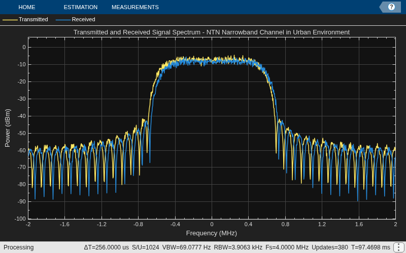
Compare the transmitted and received spectra. Because the channel introduces flat fading across the signal bandwidth, the received spectrum retains the shape of the transmitted spectrum. The Compare Channel Frequency Selectivity section compares this behavior with the frequency-selective fading observed in the NTN CDL and NTN TDL channels.

ntnNarrowbandAnalyzer = spectrumAnalyzer( ...
    SampleRate = ntnNarrowbandChan.SampleRate);
ntnNarrowbandAnalyzer.Title = "Transmitted and Received Signal Spectrum - NTN Narrowband Channel in " ...
    + string(ntnNarrowbandChan.Environment) + " Environment";
ntnNarrowbandAnalyzer.ShowLegend = true;
ntnNarrowbandAnalyzer.ChannelNames = ["Transmitted","Received"];
ntnNarrowbandAnalyzer([narrowbandSignal narrowbandOut])

NTN CDL Channel

This example supports the four channel profiles of the NTN CDL channel defined in 3GPP TR 38.811 section 6.9.1 [1]. These four channel profiles are:

NTN-CDL-A
NTN-CDL-B
NTN-CDL-C
NTN-CDL-D

The 3GPP specification defines the NTN-CDL-A and NTN-CDL-B channel profiles for non-line-of-sight (NLOS) conditions, and the NTN-CDL-C and NTN-CDL-D channel profiles for line-of-sight (LOS) conditions. The specification defines all four channel profiles at an elevation angle of 50 degrees. These are the key distinguishing factors between the NTN CDL channel [1] and the terrestrial CDL channel [2], which primarily arise due to the large propagation delay and different scattering environment in NTN scenarios.

Angle of departure — In the NTN CDL channel, the azimuth angle of departure and zenith angle of departure from the satellite (the transmitter) are the same for all clusters, whereas, in the terrestrial CDL channel, these angles can differ for each cluster.
Angular spread — In the NTN CDL channel, the azimuth spread of departure and zenith spread of departure from the satellite are zero. This means that you can effectively represent all departure rays using a single departure ray. In contrast, the terrestrial CDL channel has non-zero angular spreads.
Doppler shift — The NTN CDL channel accounts for the time evolution of Doppler shift caused by both satellite motion and UE movement. The terrestrial CDL channel, however, considers only the Doppler shift due to UE movement.
Delay profile — The NTN CDL channel delay profiles contain fewer clusters compared to those of the terrestrial CDL channel.

Follow these steps to model the NTN frequency selective fading CDL channel, as specified in 3GPP TR 38.811 section 6.9.1 [1].

Set channel parameters specific to the NTN frequency selective fading CDL channel.
Generate the NTN frequency selective fading CDL channel.
Visualize the spectrum of the faded or filtered signal.

Set NTN CDL Channel Parameters

Set the NTN frequency selective fading CDL channel parameters using the defined common parameters and the parameters specific to the NTN CDL channel. By default, this example models a downlink channel (in which the satellite is the transmitter and the UE is the receiver). To model an uplink channel, use the swapTransmitAndReceive function to reverse the link direction of nrCDLChannel before calling the step function.

% Initialize the NTN CDL channel
ntnCDLChan = nrCDLChannel;
ntnCDLChan.DelayProfile = "NTN-CDL-A";
ntnCDLChan.DelaySpread = 30e-9;                                   % In s
ntnCDLChan.SatelliteElevationAngle = commonParams.ElevationAngle;
ntnCDLChan.CarrierFrequency = commonParams.CarrierFrequency;
ntnCDLChan.SampleRate = cdlSampleRate;
ntnCDLChan.RandomStream = commonParams.RandomStream;
ntnCDLChan.Seed = commonParams.Seed;

% Set the antenna configuration
% The number of elements of an array is the product of all the elements in
% the Size field. Size is a five-element vector of form [M N P Mg Ng],
% where M is the number of rows in the antenna array, N is the number of
% columns in the antenna array, P is the number of polarizations, and Mg
% and Ng are the number of rows and columns of the array panels,
% respectively. The Element field defines the antenna element in the array.
ntnCDLChan.TransmitAntennaArray.Size = [1 1 1 1 1];
ntnCDLChan.TransmitAntennaArray.PolarizationAngles = 0;
ntnCDLChan.TransmitAntennaArray.Element = "38.901";
ntnCDLChan.ReceiveAntennaArray.Size = [1 1 2 1 1];
ntnCDLChan.ReceiveAntennaArray.PolarizationAngles = [45 -45];
ntnCDLChan.ReceiveAntennaArray.Element = "isotropic";

Use the info object function to observe the path delays, average path gains, arrival angles, departure angles, and the K-factor first tap value. Use this information to verify that the channel has been configured for the defined NTN channel delay profile and delay spread.

cdlChanInfo = info(ntnCDLChan)

cdlChanInfo = struct with fields:
    KFactorFirstCluster: -Inf
           ClusterTypes: {'NLOS'  'NLOS'  'NLOS'}
             PathDelays: [0 3.2433e-08 8.5248e-08]
       AveragePathGains: [0 -4.6750 -6.4820]
              AnglesAoD: [0 0 0]
              AnglesAoA: [178.8000 -115.7000 111.5000]
              AnglesZoD: [140 140 140]
              AnglesZoA: [35.6000 22.9000 127.4000]
    ClusterAngleSpreads: [0 15 0 7]
                    XPR: 10
    NumTransmitAntennas: 1
        NumInputSignals: 1
     NumReceiveAntennas: 2
       NumOutputSignals: 2
     ChannelFilterDelay: 7
    MaximumChannelDelay: 13

Use the MaximumDopplerShift and UTDirectionOfTravel properties to model Doppler shift in the NTN CDL channel.

The Doppler shift due to satellite motion is translated as a frequency shift, as there is no spread in departure angles. Set the second element of the MaximumDopplerShift property to the Doppler shift caused by satellite motion. Then, set the second column of the UTDirectionOfTravel property to the corresponding departure angles.
The movement of the UE introduces a Doppler or frequency spread due to a scattering environment. To model the frequency spread, set the first element of the MaximumDopplerShift property to the maximum Doppler shift due to UE movement. Then, specify the first column of the UTDirectionOfTravel property to define the direction of UE movement.

ntnCDLChan.MaximumDopplerShift = [mobileMaxDoppler satelliteDopplerShift];
ntnCDLChan.UTDirectionOfTravel = [0 cdlChanInfo.AnglesAoD(1); 90 cdlChanInfo.AnglesZoD(1)];
% Orient the transmit beam in the direction of the departure angle
ntnCDLChan.TransmitArrayOrientation = [cdlChanInfo.AnglesAoD(1); cdlChanInfo.AnglesZoD(1)-90; 0];

Generate NTN CDL Channel

Apply channel filtering to the selected transmit waveform using the path gains of the NTN frequency selective fading CDL channel.

[cdlOut,cdlPathGains,cdlSampleTimes] = ntnCDLChan(cdlSignal);

Visualize NTN CDL Channel Effect

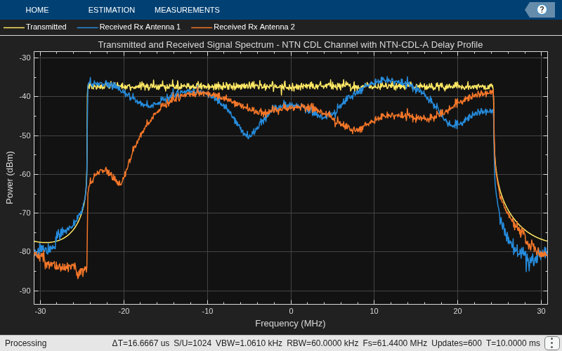
Compare the transmitted and received spectra. Unlike the flat-fading NTN narrowband channel, the frequency-selective NTN CDL channel attenuates different portions of the signal spectrum by different amounts. This behavior becomes visible only when the signal bandwidth is comparable to the channel coherence bandwidth. Therefore, use the wideband 5G waveform to observe frequency-selective shaping across the occupied band. In contrast, the occupied bandwidth of the DVB-S2X waveform is much smaller than the channel coherence bandwidth, so the channel appears flat across the signal band. The Compare Channel Frequency Selectivity section derives the channel response directly from the path gains and demonstrates the selectivity independently of the waveform.

ntnCDLAnalyzer = spectrumAnalyzer(SampleRate = ntnCDLChan.SampleRate);
ntnCDLAnalyzer.Title = "Transmitted and Received Signal Spectrum - NTN CDL Channel with " ...
    + string(ntnCDLChan.DelayProfile) + " Delay Profile";
ntnCDLAnalyzer.ShowLegend = true;
ntnCDLAnalyzer.ChannelNames = ["Transmitted", ...
    "Received Rx Antenna " + (1:size(cdlOut,2))];
ntnCDLAnalyzer([cdlSignal cdlOut])

NTN TDL Channel

This example supports the four channel profiles of the NTN TDL channel defined in 3GPP TR 38.811 section 6.9.2 [1]. These four channel profiles are:

NTN-TDL-A
NTN-TDL-B
NTN-TDL-C
NTN-TDL-D

The 3GPP specification defines the NTN-TDL-A and NTN-TDL-B channel profiles for NLOS conditions, and the NTN-TDL-C and NTN-TDL-D channel profiles for LOS conditions. The specification defines all four channel profiles at an elevation angle of 50 degrees. These are the key distinguishing factors between the NTN TDL channel [1] and the terrestrial TDL channel [2], which primarily arise due to the large propagation delay and different scattering environment in NTN scenarios.

Doppler shift — The NTN TDL channel accounts for the time evolution of Doppler shift caused by both satellite motion and UE movement. The terrestrial TDL channel, however, considers only the Doppler shift due to UE movement.
Delay profile — The NTN TDL channel delay profiles contain fewer clusters compared to those of the terrestrial TDL channel.

Follow these steps to model the NTN frequency selective fading TDL channel, as specified in 3GPP TR 38.811 section 6.9.2 [1].

Set channel parameters specific to the NTN frequency selective fading TDL channel.
Generate the NTN frequency selective fading TDL channel.
Visualize the spectrum of the faded or filtered signal.

Set NTN TDL Channel Parameters

Set the NTN frequency selective fading TDL channel parameters using the defined common parameters and the parameters specific to the NTN TDL channel. By default, this example models a downlink channel (in which the satellite is the transmitter and the UE is the receiver). To model an uplink channel, use the swapTransmitAndReceive function to reverse the link direction of nrTDLChannel before calling the step function.

% Initialize the NTN TDL channel
ntnTDLChan = nrTDLChannel;
ntnTDLChan.DelayProfile = "NTN-TDL-A";
ntnTDLChan.DelaySpread = 30e-9;                          % In s
ntnTDLChan.TransmissionDirection = "Downlink";
ntnTDLChan.MIMOCorrelation = "Low";
ntnTDLChan.Polarization = "Co-Polar";
ntnTDLChan.SampleRate = tdlSampleRate;
ntnTDLChan.MaximumDopplerShift = mobileMaxDoppler;
ntnTDLChan.SatelliteDopplerShift = satelliteDopplerShift;
ntnTDLChan.RandomStream = commonParams.RandomStream;
ntnTDLChan.Seed = commonParams.Seed;

% Set the antenna configuration

% Specify these properties, when MIMOCorrelation is a value other than
% Custom
if ~strcmpi(ntnTDLChan.MIMOCorrelation,"Custom")
    ntnTDLChan.NumTransmitAntennas = 1;
    ntnTDLChan.NumReceiveAntennas = 2;
else
    % Specify these properties, when MIMOCorrelation is Custom and
    % Polarization is Co-Polar or Cross-Polar
    if any(strcmpi(ntnTDLChan.Polarization,["Co-Polar","Cross-Polar"]))
        ntnTDLChan.TransmitCorrelationMatrix = 1;
        ntnTDLChan.ReceiveCorrelationMatrix = [1 0; 0 1];
    end
    % Specify these properties, when MIMOCorrelation is Custom and
    % Polarization is Cross-Polar
    if strcmpi(ntnTDLChan.Polarization,"Cross-Polar")
        ntnTDLChan.TransmitPolarizationAngles = [45 -45];        % In degrees
        ntnTDLChan.ReceivePolarizationAngles = [90 0];           % In degrees
        ntnTDLChan.XPR = 10;                                     % In dB
    end
    % Specify this property, when both MIMOCorrelation and Polarization are
    % Custom
    if strcmpi(ntnTDLChan.Polarization,"Custom")
        ntnTDLChan.SpatialCorrelationMatrix = [1 0; 0 1];
    end
end

Check that the channel has been configured for the defined NTN channel delay profile and delay spread by calling the object function info to observe the path delays, average path gains, and K-factor first tap value.

tdlChanInfo = info(ntnTDLChan)

tdlChanInfo = struct with fields:
          ChannelFilterDelay: 2
         MaximumChannelDelay: 8
                  PathDelays: [0 3.2433e-08 8.5248e-08]
            AveragePathGains: [0 -4.6750 -6.4820]
             KFactorFirstTap: -Inf
         NumTransmitAntennas: 1
          NumReceiveAntennas: 2
    SpatialCorrelationMatrix: [2×2 double]

Generate NTN TDL Channel

Apply channel filtering to the selected transmit waveform using the path gains of the NTN frequency selective fading TDL channel. When you select the wideband 5G waveform, its bandwidth exceeds the channel coherence bandwidth and the TDL channel imposes visible frequency selective shaping.

[tdlOut,tdlPathGains,tdlSampleTimes] = ntnTDLChan(tdlSignal);

Visualize NTN TDL Channel Effect

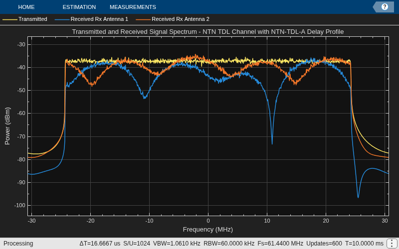
Compare the transmitted and received spectra. As with the NTN CDL channel, the frequency-selective NTN TDL channel shapes the signal band unevenly across frequency. When you select the wideband 5G waveform, whose bandwidth is comparable to the channel coherence bandwidth, you can see notches and ripples across the received spectrum. In contrast, when you use the narrowband DVB-S2X waveform, the channel exhibits a flat response across the occupied band.

ntnTDLAnalyzer = spectrumAnalyzer(SampleRate = ntnTDLChan.SampleRate);
ntnTDLAnalyzer.Title = "Transmitted and Received Signal Spectrum - NTN TDL Channel with " ...
    + string(ntnTDLChan.DelayProfile) + " Delay Profile";
ntnTDLAnalyzer.ShowLegend = true;
ntnTDLAnalyzer.ChannelNames = ["Transmitted", ...
    "Received Rx Antenna " + (1:size(tdlOut,2))];
ntnTDLAnalyzer([tdlSignal tdlOut])

Compare Channel Frequency Selectivity

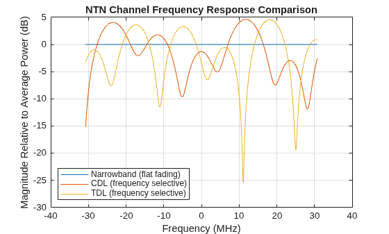
The narrowband, CDL, and TDL channels differ in how their gain varies across frequency. Derive the channel frequency response $H (f) = \sum_{k} g_{k} e^{- j 2 π f τ_{k}}$ directly from the path gains $g_{k}$ and path delays $τ_{k}$ of each channel. Deriving the response from the channel rather than from a filtered waveform isolates the channel frequency shaping from the transmit signal. Because $H (f)$ depends only on the physical path delays, the responses of all three channels can be evaluated on a common frequency grid even though the channels operate at different sample rates.

Evaluate the response over the widest channel bandwidth so that the narrowband channel response appears within the comparison range. Note that these plots depict the instantaneous channel and do not represent the average channel realizations.

freqSpan = max([ntnNarrowbandChan.SampleRate ntnCDLChan.SampleRate ntnTDLChan.SampleRate]);
freqGrid = linspace(-freqSpan/2,freqSpan/2,1024).';

Overlay Channel Frequency Responses

Overlay the frequency response magnitude of the three channels, with each response referenced to its own average power so that the comparison reflects the shape across frequency rather than absolute path loss. The narrowband channel is flat across the band because it has a single path, whereas the CDL and TDL channels exhibit deep notches and ripples that are the signature of frequency selective fading. The plot shows the channel response of first transmit and receive antenna pair.

narrowbandResponse = channelFrequencyResponse(narrowbandPathGains,p681ChannelInfo.PathDelays,freqGrid);
cdlResponse = channelFrequencyResponse(cdlPathGains,cdlChanInfo.PathDelays,freqGrid);
tdlResponse = channelFrequencyResponse(tdlPathGains,tdlChanInfo.PathDelays,freqGrid);

% Reference each response to its own average power, so 0 dB marks the
% average-power gain for every channel. Averaging the linear power (|H|^2)
% and taking decibels once keeps the reference independent of notch depth,
% which a mean of the per-sample dB values would not achieve.
narrowbandMagnitude = mag2db(abs(narrowbandResponse)/rms(narrowbandResponse));
cdlMagnitude = mag2db(abs(cdlResponse)/rms(cdlResponse));
tdlMagnitude = mag2db(abs(tdlResponse)/rms(tdlResponse));

figure
plot(freqGrid*1e-6,narrowbandMagnitude)
hold on
plot(freqGrid*1e-6,cdlMagnitude)
plot(freqGrid*1e-6,tdlMagnitude)
hold off
xlabel("Frequency (MHz)")
ylabel("Magnitude Relative to Average Power (dB)")
title("NTN Channel Frequency Response Comparison")
legend("Narrowband (flat fading)","CDL (frequency selective)", ...
    "TDL (frequency selective)",Location="southwest")
grid on

Figure contains an axes object. The axes object with title NTN Channel Frequency Response Comparison, xlabel Frequency (MHz), ylabel Magnitude Relative to Average Power (dB) contains 3 objects of type line. These objects represent Narrowband (flat fading), CDL (frequency selective), TDL (frequency selective).

Mesh Time-Frequency Response of Each Channel

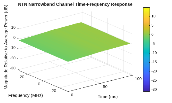
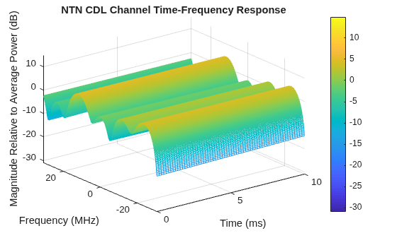
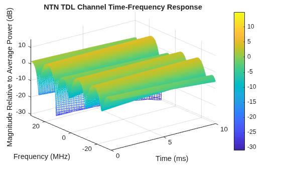
The overlay shows the response at a single time instant. Because the channels are time varying, evaluate $H (f)$ at every path-gain snapshot to form a time-frequency surface. Reference each surface to its own average power and plot all three on a common amplitude scale, so that the narrowband channel appears as a nearly flat plane while the CDL and TDL surfaces show notches of comparable, directly readable depth. The narrowband channel is flat along frequency and undulates only slowly over time, reflecting the slow flat fading of the land mobile-satellite channel. The CDL and TDL surfaces are corrugated along frequency, and the notches drift over time because of the Doppler shift. The plot shows the time-frequency response of first transmit-receive antenna pair.

[narrowbandSurface,narrowbandMeshTimes] = channelTimeFrequencyResponse( ...
    narrowbandPathGains,p681ChannelInfo.PathDelays,narrowbandSampleTimes,freqGrid);
[cdlSurface,cdlMeshTimes] = channelTimeFrequencyResponse( ...
    cdlPathGains,cdlChanInfo.PathDelays,cdlSampleTimes,freqGrid);
[tdlSurface,tdlMeshTimes] = channelTimeFrequencyResponse( ...
    tdlPathGains,tdlChanInfo.PathDelays,tdlSampleTimes,freqGrid);

% Derive one amplitude scale from all three surfaces so the plots share the
% same z-axis and color resolution. Referencing to average power makes the
% deviations asymmetric: peaks rise only a few decibels above 0 dB while
% notches plunge far below it. Set separate upper and lower limits so the
% axis avoids empty range, and floor the lower limit because a single deep
% null drives mag2db toward negative infinity.
allSurfaces = [narrowbandSurface(:); cdlSurface(:); tdlSurface(:)];
meshUpperLimit = max(allSurfaces)+10;
meshLowerLimit = max(min(allSurfaces),-40);
meshAmplitudeLimits = [meshLowerLimit meshUpperLimit];

meshChannelTimeFrequencyResponse(narrowbandMeshTimes,freqGrid,narrowbandSurface, ...
    meshAmplitudeLimits,"NTN Narrowband Channel Time-Frequency Response")

Figure contains an axes object. The axes object with title NTN Narrowband Channel Time-Frequency Response, xlabel Time (ms), ylabel Frequency (MHz) contains an object of type surface.

meshChannelTimeFrequencyResponse(cdlMeshTimes,freqGrid,cdlSurface, ...
    meshAmplitudeLimits,"NTN CDL Channel Time-Frequency Response")

Figure contains an axes object. The axes object with title NTN CDL Channel Time-Frequency Response, xlabel Time (ms), ylabel Frequency (MHz) contains an object of type surface.

meshChannelTimeFrequencyResponse(tdlMeshTimes,freqGrid,tdlSurface, ...
    meshAmplitudeLimits,"NTN TDL Channel Time-Frequency Response")

Figure contains an axes object. The axes object with title NTN TDL Channel Time-Frequency Response, xlabel Time (ms), ylabel Frequency (MHz) contains an object of type surface.

Further Exploration

You can use this example to further explore these options:

To configure and analyze the NTN narrowband, TDL, or CDL channels for other satellite orbits, change the SatelliteAltitude field of the commonParams structure.
To analyze the NTN flat fading narrowband channel for another environment, change the Environment property of the p681LMSChannel.
To analyze the NTN TDL channel for LOS delay profiles, change the DelayProfile property of the nrTDLChannel to NTN-TDL-C or NTN-TDL-D.
To configure the NTN TDL channel for multiple antennas, change the MIMOCorrelation and Polarization properties of the nrTDLChannel. You might need to set other properties depending on these values.
To analyze the NTN CDL channel for LOS delay profiles with multiple antennas, set the DelayProfile property of nrCDLChannel to NTN-CDL-C or NTN-CDL-D, and adjust the Size field of the TransmitAntennaArray or ReceiveAntennaArray property.
Use the NTN channel models in a link simulation to compute the link metric. For more information, see the NR NTN PDSCH Throughput example.
To obtain different channel realizations for analysis, change the Seed field in the commonParams structure.

References

[1] 3GPP TR 38.811. "Study on new radio (NR) to support non-terrestrial networks." 3rd Generation Partnership Project; Technical Specification Group Radio Access Network.

[2] 3GPP TR 38.901. "Study on channel model for frequencies from 0.5 to 100 GHz." 3rd Generation Partnership Project; Technical Specification Group Radio Access Network.

[3] 3GPP TR 38.821. "Solutions for NR to support non-terrestrial networks (NTN)." 3rd Generation Partnership Project; Technical Specification Group Radio Access Network.

[4] ITU-R Recommendation P.681-11 (08/2019). "Propagation data required for the design systems in the land mobile-satellite service." P Series; Radio wave propagation.

Supporting Functions

The example uses these supporting functions.

function [out,fs] = parseSignalAndSampleRate(sigType,nrIn,nrFs,dvbIn,dvbFs)
% Select the transmit signal and its sample rate for each channel. Each
% channel provides an independent signal selection. The narrowband channel
% uses the DVB-S2X waveform, while the CDL and TDL channels use the
% wideband 5G waveform in the same simulation run. Configure each channel
% with the sample rate of its corresponding waveform.
    if contains(sigType,"DVB")
        out = dvbIn;
        fs = dvbFs;
    else
        out = nrIn;
        fs = nrFs;
    end
end

function freqResponse = channelFrequencyResponse(pathGains,pathDelays,freqGrid)
% Evaluate the channel frequency response H(f) = sum_k g_k
% exp(-j2*pi*f*tau_k) at the midpoint time snapshot, from the first
% transmit-receive antenna pair. The midpoint snapshot preserves the deep
% frequency notches that Doppler-induced motion would blur when averaged
% over time. Deriving H(f) from the path gains and delays isolates the
% channel frequency shaping from any transmit waveform, so the same
% function serves the flat narrowband channel (single tap, flat response)
% and the frequency selective CDL and TDL channels.
    numTaps = numel(pathDelays);
    midSnapshot = round(size(pathGains,1)/2);
    % Index by dimension explicitly so the tap axis survives the single-tap
    % narrowband channel, where a squeeze would collapse it away
    tapGains = reshape(pathGains(midSnapshot,1:numTaps,1,1),numTaps,1);
    freqResponse = exp(-1j*2*pi*freqGrid*pathDelays(:).')*tapGains;
end

function [surfaceMagnitude,snapshotTimes] = channelTimeFrequencyResponse(pathGains,pathDelays,sampleTimes,freqGrid)
% Evaluate the channel frequency response magnitude over both frequency and
% time. Evaluating H(f) at every path-gain snapshot shows how the frequency
% response evolves: the flat narrowband channel stays flat along frequency,
% while the selective channels show notches that drift over time due to
% Doppler. This function references each surface to its own average power so
% that the comparison reflects the shape across frequency and time rather
% than absolute path loss, matches the convention the overlay plot uses, and
% lets all channels share a common amplitude scale when plotted.

    % Use a coarse time grid to keep the surface legible and the figure
    % compact. Although the channels report thousands of snapshots, a
    % coarse grid captures the time evolution just as clearly.
    maxTimeSnapshots = 64;
    numSnapshots = size(pathGains,1);
    snapshotIdx = unique(round(linspace(1,numSnapshots,min(maxTimeSnapshots,numSnapshots))));

    numTaps = numel(pathDelays);
    numUpdatedSnaps = numel(snapshotIdx);
    delayPhase = exp(-1j*2*pi*freqGrid*pathDelays(:).');    % [numFreq x numTaps]
    surfaceLinear = zeros(numel(freqGrid),numUpdatedSnaps);
    for n = 1:numUpdatedSnaps
        tapGains = reshape(pathGains(snapshotIdx(n),1:numTaps,1,1),numTaps,1);
        surfaceLinear(:,n) = abs(delayPhase*tapGains);
    end
    % Reference to the average power over the whole surface, then convert to
    % decibels once. Averaging the linear power keeps the 0 dB reference
    % independent of notch depth, which a mean of the per-sample dB values
    % would not achieve.
    surfaceMagnitude = mag2db(surfaceLinear/rms(surfaceLinear(:)));
    snapshotTimes = sampleTimes(snapshotIdx);
end

function meshChannelTimeFrequencyResponse(snapshotTimes,freqGrid,surfaceMagnitude,amplitudeLimits,titleText)
% Plot a channel time-frequency response surface on a shared amplitude
% scale. Fixing the z-axis and color limits to the same range for every
% channel preserves the relative magnitudes across the three separate
% figures, so the flat narrowband plane and the corrugated CDL and TDL
% surfaces read on one consistent scale. amplitudeLimits gives the
% two-element [lower upper] range that all channels share.
    figure
    mesh(snapshotTimes*1e3,freqGrid*1e-6,surfaceMagnitude)
    xlabel("Time (ms)")
    ylabel("Frequency (MHz)")
    zlabel("Magnitude Relative to Average Power (dB)")
    title(titleText)
    zlim(amplitudeLimits)
    clim(amplitudeLimits)
    colorbar
    view(-37.5,30)
end