Main Content

sdlsim

Time response of sampled-data feedback system

Syntax

sdlsim(p,k,w,t,tf)
sdlsim(p,k,w,t,tf,x0,z0)
sdlsim(p,k,w,t,tf,x0,z0,int)
[vt,yt,ut,t] = sdlsim(p,k,w,t,tf)
[vt,yt,ut,t] = sdlsim(p,k,w,t,tf,x0,z0,int)

Description

sdlsim(p,k,w,t,tf) plots the time response of the hybrid feedback system. lft(p,k), is forced by the continuous input signal described by w and t (values and times, as in lsim). p must be a continuous-time LTI system, and k must be discrete-time LTI system with a specified sample time (the unspecified sample time –1 is not allowed). The final time is specified with tf.

sdlsim(p,k,w,t,tf,x0,z0) specifies the initial state vector x0 of p, and z0 of k, at time t(1).

sdlsim(p,k,w,t,tf,x0,z0,int) specifies the continuous-time integration step size int. sdlsim forces int = (k.Ts)/N int where N>4 is an integer. If any of these optional arguments is omitted, or passed as empty matrices, then default values are used. The default value for x0 and z0 is zero. Nonzero initial conditions are allowed for p (and/or k) only if p (and/or k) is an ss object.

If p and/or k is an LTI array with consistent array dimensions, then the time simulation is performed pointwise across the array dimensions.

[vt,yt,ut,t] = sdlsim(p,k,w,t,tf) computes the continuous-time response of the hybrid feedback system lft(p,k) forced by the continuous input signal defined by w and t (values and times, as in lsim). p must be a continuous-time system, and k must be discrete-time, with a specified sample time (the unspecified sample time –1 is not allowed). The final time is specified with tf. The outputs vt, yt and ut are 2-by-1 cell arrays: in each the first entry is a time vector, and the second entry is the signal values. Stored in this manner, the signal vt is plotted by using one of the following commands:

plot(vt{1},vt{2})
plot(vt{:}) 

Signals yt and ut are respectively the input to k and output of k.

If p and/or k are LTI arrays with consistent array dimensions, then the time simulation is performed pointwise across the array dimensions. The outputs are 2-by-1-by-array dimension cell arrays. All responses can be plotted simultaneously, for example, plot(vt).

[vt,yt,ut,t] = sdlsim(p,k,w,t,tf,x0,z0,int) The optional arguments are int (integration step size), x0 (initial condition for p), and z0 (initial condition for k). sdlsim forces int = (k.Ts)/N, where N>4 is an integer. If any of these arguments is omitted, or passed as empty matrices, then default values are used. The default value for x0 and z0 is zero. Nonzero initial conditions are allowed for p (and/or k) only if p (and/or k) is an ss object.

Examples

collapse all

To illustrate the use of sdlsim, consider the application of a discrete controller to a plant with an integrator and near integrator. A continuous plant and a discrete controller are created. A sample-and-hold equivalent of the plant is formed and the discrete closed-loop system is calculated. Simulating this gives the system response at the sample points. sdlsim is then used to calculate the intersample behavior.

P = tf(1,[1, 1e-5,0]); 
T = 1.0/20; 
C = ss([-1.5 T/4; -2/T -.5],[ .5 2;1/T 1/T],... 
   [-1/T^2  -1.5/T], [1/T^2  0],T); 
Pd = c2d(P,T,'zoh');

Use connect to construct the interconnected feedback system.

C.InputName = {'ref','y'};
C.OutputName = 'u';
Pd.Inputname = 'u';
Pd.OutputName = 'y';
dclp = connect(C,Pd,'ref','y');

Use step to simulate the digital step response.

[yd,td] = step(dclp,20*T);

Set up the continuous interconnection and calculate the sampled data response with sdlsim.

M = [0,1;1,0;0,1]*blkdiag(1,P); 
t = [0:.01:1]'; 
u = ones(size(t)); 
y1 = sdlsim(M,C,u,t); 
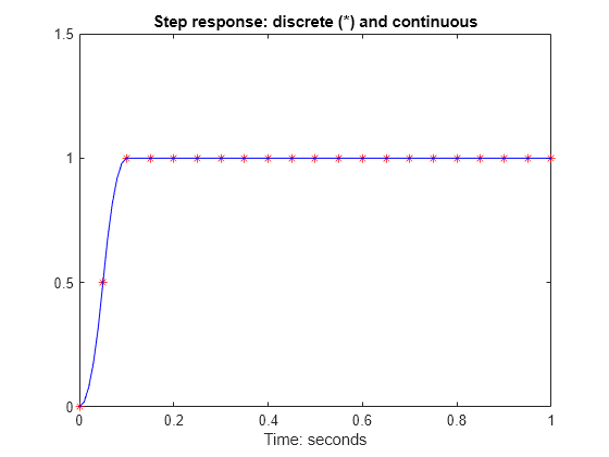
plot(td,yd,'r*',y1{:},'b-') 
axis([0,1,0,1.5]) 
xlabel('Time: seconds') 
title('Step response: discrete (*) and continuous')

Figure contains an axes object. The axes object with title Step response: discrete (*) and continuous, xlabel Time: seconds contains 2 objects of type line. One or more of the lines displays its values using only markers

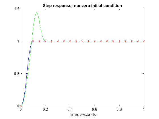
You can see the effect of a nonzero initial condition in the continuous-time system. Note how examining the system at only the sample points will underestimate the amplitude of the overshoot.

y2 = sdlsim(M,C,u,t,1,0,[0.25;0]); 
plot(td,yd,'r*',y1{:},'b-',y2{:},'g--') 
axis([0,1,0,1.5]) 
xlabel('Time: seconds') 
title('Step response: nonzero initial condition')

Figure contains an axes object. The axes object with title Step response: nonzero initial condition, xlabel Time: seconds contains 3 objects of type line. One or more of the lines displays its values using only markers

Finally, you can examine the effect of a sinusoidal disturbance at the continuous-time plant output. This controller is not designed to reject such a disturbance and the system does not contain antialiasing filters. Simulating the effect of antialiasing filters is easily accomplished by including them in the continuous interconnection structure.

M2 = [0,1,1;1,0,0;0,1,1]*blkdiag(1,1,P); 
t = [0:.001:1]'; 
dist = 0.1*sin(41*t); 
u = ones(size(t)); 
[y3,meas,act] = sdlsim(M2,C,[u dist],t,1); 
plot(y3{:},'-',t,dist,'b--',t,u,'g-.') 
xlabel('Time: seconds') 
title('Step response: disturbance (dashed) and  output (solid)')

Figure contains an axes object. The axes object with title Step response: disturbance (dashed) and output (solid), xlabel Time: seconds contains 3 objects of type line.

Algorithms

sdlsim oversamples the continuous-time, N times the sample rate of the controller k.

Version History

Introduced before R2006a
Go to top of page