Main Content

derivative

Time derivative of manipulator model states

Since R2019b

Description

example

stateDot = derivative(taskMotionModel,state,refPose,refVel) computes the time derivative of the task-space motion model based on the current state and desired end-effector pose and velocities.

stateDot = derivative(taskMotionModel,state,refPose,refVel,fExt) computes the time derivative of the task-space motion model with external forces on the manipulator.

example

stateDot = derivative(jointMotionModel,state,cmds) computes the time derivative of the joint-space motion model based on the current state and motion commands.

stateDot = derivative(jointMotionModel,state,cmds,fExt) computes the time derivative of the joint-space motion model with external forces on the manipulator using a joint-space model.

Examples

collapse all

This example shows how to create and use a jointSpaceMotionModel object for a manipulator robot in joint-space.

Create the Robot

robot = loadrobot("kinovaGen3","DataFormat","column","Gravity",[0 0 -9.81]);

Set Up the Simulation

Set the timespan to be 1 s with a timestep size of 0.01 s. Set the initial state to be the robots, home configuration with a velocity of zero.

tspan = 0:0.01:1;
initialState = [homeConfiguration(robot); zeros(7,1)];

Define the reference state with a target position, zero velocity, and zero acceleration.

targetState = [pi/4; pi/3; pi/2; -pi/3; pi/4; -pi/4; 3*pi/4; zeros(7,1); zeros(7,1)];

Create the Motion Model

Model the system with computed torque control and error dynamics defined by a moderately fast step response with 5% overshoot.

motionModel = jointSpaceMotionModel("RigidBodyTree",robot);
updateErrorDynamicsFromStep(motionModel,.3,.05);

Simulate the Robot

Use the derivative function of the model as the input to the ode45 solver to simulate the behavior over 1 second.

[t,robotState] = ode45(@(t,state)derivative(motionModel,state,targetState),tspan,initialState);

Plot the Response

Plot the positions of all the joints actuating to their target state. Joints with a higher displacement between the starting position and the target position actuate to the target at a faster rate than those with a lower displacement. This leads to an overshoot, but all of the joints have the same settling time.

figure
plot(t,robotState(:,1:motionModel.NumJoints));
hold all;
plot(t,targetState(1:motionModel.NumJoints)*ones(1,length(t)),"--");
title("Joint Position (Solid) vs Reference (Dashed)");
xlabel("Time (s)")
ylabel("Position (rad)");

This example shows how to create and use a taskSpaceMotionModel object for a manipulator robot arm in task-space.

Create the Robot

robot = loadrobot("kinovaGen3","DataFormat","column","Gravity",[0 0 -9.81]);

Set Up the Simulation

Set the time span to be 1 second with a timestep size of 0.02 seconds. Set the initial state to the home configuration of the robot, with a velocity of zero.

tspan = 0:0.02:1;
initialState = [homeConfiguration(robot);zeros(7,1)];

Define a reference state with a target position and zero velocity.

refPose = trvec2tform([0.6 -.1 0.5]);
refVel = zeros(6,1);

Create the Motion Model

Model the behavior as a system under proportional-derivative (PD) control.

motionModel = taskSpaceMotionModel("RigidBodyTree",robot,"EndEffectorName","EndEffector_Link");

Simulate the Robot

Simulate the behavior over 1 second using a stiff solver to more efficiently capture the robot dynamics. Using ode15s enables higher precision around the areas with a high rate of change.

[t,robotState] = ode15s(@(t,state)derivative(motionModel,state,refPose,refVel),tspan,initialState);

Plot the Response

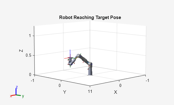
Plot the robot's initial position and mark the target with an X.

figure
show(robot,initialState(1:7));
hold all
plot3(refPose(1,4),refPose(2,4),refPose(3,4),"x","MarkerSize",20)

Observe the response by plotting the robot in a 5 Hz loop.

r = rateControl(5);
for i = 1:size(robotState,1)
    show(robot,robotState(i,1:7)',"PreservePlot",false);
    waitfor(r);
end

Input Arguments

collapse all

Task-space motion model, specified as a taskSpaceMotionModel object, which defines the properties of the motion model.

Joint-space motion model, specified as a jointSpaceMotionModel object, which defines the properties of the motion model.

Joint positions and velocities, specified as a 2n-element column vector of the form [q; qDot]. n is the number of non-fixed joints in the associated rigidBodyTree of the motion model. q, represents the position of each joint, specified in radians. qDot represents the velocity of each joint, specified in radians per second.

Desired pose of the end effector in the task-space, specified as an 4-by-4 homogeneous transformation matrix. Units are in meters.

Desired velocities of the end effector in the task space, specified as a six-element column vector of the form [omega; v]. omega represents a column vector of three angular velocities about the x, y, and z axes in radians per second. v represents a column vector of three linear velocities along the x, y, and z axes in meters per second.

Control commands indicating the desired motion, specified as either a 2n-element column vector or a 3n-element column vector depending on the MotionType property of jointMotionModel:

  • "PDControl" — 2n-element column vector, [qRef; qRefDot]. qRef and qRefDot represent joint positions and joint velocities, respectively.

  • "ComputedTorqueControl" — 3n-element column vector, [qRef; qRefDot; qRefDDot]. qRef, qRefDot, and qRefDDot represent the joint positions, joint velocities, and joint accelerations, respectively.

  • "IndependentJointMotion" — 3n-element column vector, [qRef; qRefDot; qRefDDot]. qRef, qRefDot, and qRefDDot represent the joint positions, joint velocities, and joint accelerations, respectively.

External forces, specified as an 6-by-m matrix. Each row is a wrench on a rigid body, spatially transformed to the base frame, in the form [Tx Ty Tz Fx Fy Fz]. m is the number of bodies in the associated rigidBodyTree object. The first three elements of the wrench correspond to the moments around the xyz-axes in Newton-meters. The last three elements are linear forces along the same axes in Newtons.

For more information about external forces on rigid body trees and spatially transforms, see the externalForce function and Compute Joint Torques To Balance An Endpoint Force and Moment.

Output Arguments

collapse all

Time derivative based on current state and the specified control commands or reference pose and velocities, returned as a 2n-element column vector, [qDot; qDDot], where qDot is an n-element column vector of joint velocities, and qDDot is an n-element column vector of joint accelerations. n is the number of joints in the associated rigidBodyTree of the motion model.

Extended Capabilities

C/C++ Code Generation
Generate C and C++ code using MATLAB® Coder™.

Version History

Introduced in R2019b