Main Content

cubicpolytraj

Generate third-order polynomial trajectories

Description

example

[q,qd,qdd,pp] = cubicpolytraj(wayPoints,timePoints,tSamples) generates a third-order polynomial that achieves a given set of input waypoints with corresponding time points. The function outputs positions, velocities, and accelerations at the given time samples, tSamples. The function also returns the piecewise polynomial pp form of the polynomial trajectory with respect to time.

[q,qd,qdd,pp] = cubicpolytraj(___,Name,Value) specifies additional parameters as Name,Value pair arguments using any combination of the previous syntaxes.

Examples

collapse all

Use the cubicpolytraj function with a given set of 2-D xy waypoints. Time points for the waypoints are also given.

wpts = [1 4 4 3 -2 0; 0 1 2 4 3 1];
tpts = 0:5;

Specify a time vector for sampling the trajectory. Sample at a smaller interval than the specified time points.

tvec = 0:0.01:5;

Compute the cubic trajectory. The function outputs the trajectory positions (q), velocity (qd), acceleration (qdd), and polynomial coefficients (pp) of the cubic polynomial.

[q, qd, qdd, pp] = cubicpolytraj(wpts, tpts, tvec);

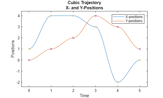
Plot the cubic trajectories for the x- and y-positions. Compare the trajectory with each waypoint.

plot(tvec, q)
hold all
plot(tpts, wpts, 'x')
xlabel('t')
ylabel('Positions')
legend('X-positions','Y-positions')
hold off

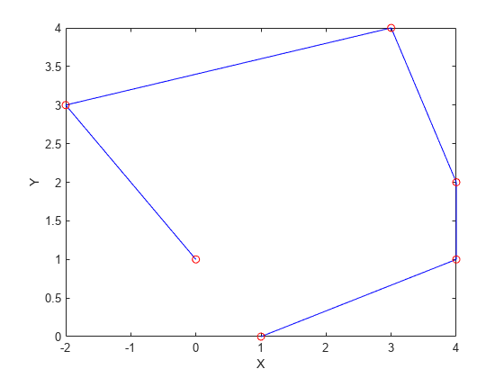
You can also verify the actual positions in the 2-D plane. Plot the separate rows of the q vector and the waypoints as x- and y -positions.

figure
plot(q(1,:),q(2,:),'-b',wpts(1,:),wpts(2,:),'or')
xlabel('X')
ylabel('Y')

Input Arguments

collapse all

Points for waypoints of trajectory, specified as an n-by-p matrix, where n is the dimension of the trajectory and p is the number of waypoints.

Example: [1 4 4 3 -2 0; 0 1 2 4 3 1]

Data Types: single | double

Time points for waypoints of trajectory, specified as a p-element vector.

Example: [0 2 4 5 8 10]

Data Types: single | double

Time samples for the trajectory, specified as an m-element vector. The output position, q, velocity, qd, and accelerations, qdd, are sampled at these time intervals.

Example: 0:0.01:10

Data Types: single | double

Name-Value Arguments

Specify optional pairs of arguments as Name1=Value1,...,NameN=ValueN, where Name is the argument name and Value is the corresponding value. Name-value arguments must appear after other arguments, but the order of the pairs does not matter.

Before R2021a, use commas to separate each name and value, and enclose Name in quotes.

Example: 'VelocityBoundaryCondition',[1 0 -1 -1 0 0; 1 1 1 -1 -1 -1]

Velocity boundary conditions for each waypoint, specified as the comma-separated pair consisting of 'VelocityBoundaryCondition' and an n-by-p matrix. Each row corresponds to the velocity at all p waypoints for the respective variable in the trajectory.

Example: [1 0 -1 -1 0 0; 1 1 1 -1 -1 -1]

Data Types: single | double

Output Arguments

collapse all

Positions of the trajectory at the given time samples in tSamples, returned as an m-element vector, where m is the length of tSamples.

Data Types: single | double

Velocities of the trajectory at the given time samples in tSamples, returned as a vector.

Data Types: single | double

Accelerations of the trajectory at the given time samples in tSamples, returned as a vector.

Data Types: single | double

Piecewise-polynomial, returned as a structure that defines the polynomial for each section of the piecewise trajectory. You can build your own piecewise polynomials using mkpp, or evaluate the polynomial at specified times using ppval. The structure contains the fields:

  • form: 'pp'.

  • breaks: p-element vector of times when the piecewise trajectory changes forms. p is the number of waypoints.

  • coefs: n(p–1)-by-order matrix for the coefficients for the polynomials. n(p–1) is the dimension of the trajectory times the number of pieces. Each set of n rows defines the coefficients for the polynomial that described each variable trajectory.

  • pieces: p–1. The number of breaks minus 1.

  • order: Degree of the polynomial + 1. For example, cubic polynomials have an order of 4.

  • dim: n. The dimension of the control point positions.

Extended Capabilities

C/C++ Code Generation
Generate C and C++ code using MATLAB® Coder™.

Version History

Introduced in R2019a