earthSurfacePermittivity

Permittivity and conductivity of earth surface materials

Since R2020a

Syntax

[epsilon,sigma,complexepsilon] = earthSurfacePermittivity("pure-water",fc,temp)

[epsilon,sigma,complexepsilon] = earthSurfacePermittivity("sea-water",fc,temp,salinity)

[epsilon,sigma,complexepsilon] = earthSurfacePermittivity("pure-ice",fc,temp)

[epsilon,sigma,complexepsilon] = earthSurfacePermittivity("wet-ice",fc,liqfrac)

[epsilon,sigma,complexepsilon] = earthSurfacePermittivity("multi-year-ice",fc,temp,avf)

[epsilon,sigma,complexepsilon] = earthSurfacePermittivity("dry-snow",fc,temp,dsd)

[epsilon,sigma,complexepsilon] = earthSurfacePermittivity("wet-snow",fc,temp,dsd,lwc)

[epsilon,sigma,complexepsilon] = earthSurfacePermittivity("soil",fc,temp,sandpercent,claypercent,sg,vwc)

[epsilon,sigma,complexepsilon] = earthSurfacePermittivity("soil",fc,temp,sandpercent,claypercent,sg,vwc,bulkdensity)

[epsilon,sigma,complexepsilon] = earthSurfacePermittivity("vegetation",fc,temp,gwc)

Description

The earthSurfacePermittivity function computes the real relative permittivity, conductivity, and complex relative permittivity of earth surface materials based on the methods and equations presented in International Telecommunication Union Recommendation (ITU-R) P.527-5 through ITU-R P.527-6 [1]. The earthSurfacePermittivity function provides various syntaxes to account for characteristics germane to the specified surface material.

Water

[epsilon,sigma,complexepsilon] = earthSurfacePermittivity("pure-water",fc,temp) calculates the real relative permittivity, conductivity, and complex relative permittivity of pure water at the specified frequency and temperature.

[epsilon,sigma,complexepsilon] = earthSurfacePermittivity("sea-water",fc,temp,salinity) calculates the real relative permittivity, conductivity, and complex relative permittivity of sea water at the specified frequency, temperature, and salinity.

Ice

[epsilon,sigma,complexepsilon] = earthSurfacePermittivity("pure-ice",fc,temp) calculates the real relative permittivity, conductivity, and complex relative permittivity of pure ice at the specified frequency and temperature.

[epsilon,sigma,complexepsilon] = earthSurfacePermittivity("wet-ice",fc,liqfrac) calculates the real relative permittivity, conductivity, and complex relative permittivity of wet ice at the specified frequency and liquid water volume fraction.

[epsilon,sigma,complexepsilon] = earthSurfacePermittivity("multi-year-ice",fc,temp,avf) calculates the real relative permittivity, conductivity, and complex relative permittivity of multi-year ice at the specified frequency, temperature, and air volume fraction. (since R2024a)

Snow

[epsilon,sigma,complexepsilon] = earthSurfacePermittivity("dry-snow",fc,temp,dsd) calculates the real relative permittivity, conductivity, and complex relative permittivity of dry snow at the specified frequency, temperature, and dry snow density. (since R2024a)

[epsilon,sigma,complexepsilon] = earthSurfacePermittivity("wet-snow",fc,temp,dsd,lwc) calculates the real relative permittivity, conductivity, and complex relative permittivity of wet snow at the specified frequency, temperature, dry snow density, and liquid water volume fraction. (since R2024a)

Soil

[epsilon,sigma,complexepsilon] = earthSurfacePermittivity("soil",fc,temp,sandpercent,claypercent,sg,vwc) calculates the real relative permittivity, conductivity, and complex relative permittivity of soil at the specified frequency, temperature, percentage of sand by volume, percentage of clay by volume, specific gravity, and volumetric water content. This syntax uses an approximation formula for the bulk density of the soil.

[epsilon,sigma,complexepsilon] = earthSurfacePermittivity("soil",fc,temp,sandpercent,claypercent,sg,vwc,bulkdensity) specifies the bulk density of the soil in addition to the input arguments from the previous syntax.

Vegetation

[epsilon,sigma,complexepsilon] = earthSurfacePermittivity("vegetation",fc,temp,gwc) calculates the real relative permittivity, conductivity, and complex relative permittivity of vegetation at the specified frequency, temperature, and gravimetric water content.

Examples

Compare Permittivity and Conductivity of Pure Water and Sea Water

Compare the real relative permittivity and conductivity of pure water and sea water.

Specify the carrier frequency as 9 GHz. Specify the temperature of the water as 30 °C.

fc = 9e9; % Hz
temp = 30; % °C

Compute the real relative permittivity and conductivity of pure water and sea water. Specify the salinity of the sea water as 35 g/kg.

[epsilon_pure,sigma_pure] = earthSurfacePermittivity("pure-water",fc,temp);
[epsilon_sea,sigma_sea] = earthSurfacePermittivity("sea-water",fc,temp,35);

Compare the real relative permittivity values.

disp("Real relative permittivity of pure water: " + epsilon_pure)

Real relative permittivity of pure water: 66.1457

disp("Real relative permittivity of sea water: " + epsilon_sea)

Real relative permittivity of sea water: 64.9968

Compare the conductivity values.

disp("Conductivity of pure water: " + sigma_pure)

Conductivity of pure water: 12.6445

disp("Conductivity of sea water: " + sigma_sea)

Conductivity of sea water: 13.183

Compare Permittivity and Conductivity of Wet Ice and Pure Ice

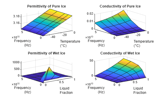
Compare the real relative permittivity and conductivity of pure ice with varying temperatures, and wet ice with varying amounts of liquid water.

Specify frequency, liquid water volume fraction, and temperature values using vectors. Create grids from the values by repeating the vectors.

freq0 = [0.1 10 20 40 60]*1e9;
freq = repmat(freq0,6,1);

liqfrac0 = 0:0.2:1;
liqfrac = repmat(liqfrac0',1,5);

temp0 = -50:10:0;
temp = repmat(temp0',1,5);

For each frequency and temperature value, calculate the permittivity and conductivity of pure ice. Apply the earthSurfacePermittivity function to each element of the gridded inputs by using the arrayfun function.

[epsilon_pure,sigma_pure] = arrayfun(@(x,y) ...
    earthSurfacePermittivity("pure-ice",x,y),freq,temp);

For each frequency and liquid water fraction value, calculate the permittivity and conductivity of wet ice.

[epsilon_wet,sigma_wet] = arrayfun(@(x,y) ...
    earthSurfacePermittivity("wet-ice",x,y),freq,liqfrac);

Display the results using multiple surface plots. Organize the plots using a tiled chart layout.

figure
tiledlayout(2,2)

nexttile
surf(temp,freq,epsilon_pure,FaceColor="interp")
title("Permittivity of Pure Ice")
xlabel(["Temperature","(°C)"])
ylabel(["Frequency","(Hz)"])

nexttile
surf(temp,freq,sigma_pure,FaceColor="interp")
title("Conductivity of Pure Ice")
xlabel(["Temperature","(°C)"])
ylabel(["Frequency","(Hz)"])

nexttile
surf(liqfrac,freq,epsilon_wet,FaceColor="interp")
title("Permittivity of Wet Ice")
xlabel(["Liquid","Fraction"])
ylabel(["Frequency","(Hz)"])

nexttile
surf(liqfrac,freq,sigma_wet,FaceColor="interp")
title("Conductivity of Wet Ice")
xlabel(["Liquid","Fraction"])
ylabel(["Frequency","(Hz)"])

Calculate Permittivity and Conductivity of Soil Mixtures

Calculate the real relative permittivity and conductivity of several soil mixtures.

Specify the carrier frequency, the temperature of the soil, and the volumetric water content of the soil.

fc = 28e9; % Hz
temp = 23; % °C
vwc = 0.5; 

ITU-R P.527-6 defines textual classifications for different types of soil. These classifications depend on the percentages of sand, clay, and silt in the soils. Using values from Table 2 in ITU-R P.527-6, specify representative percentages of sand and clay for sandy loam, loam, silty loam, and silty clay. Use these values to calculate the percentages of silt.

soilType = ["Sandy Loam","Loam","Silty Loam","Silty Clay"]';
percentSand = [51.52 41.96 30.63 5.02]';
percentClay = [13.42 8.53 13.48 47.38]';
percentSilt = 100 - (percentSand + percentClay);

Using values from Table 2 in ITU-R P.527-6, specify representative values for the specific gravity and bulk density of sandy loam, loam, silty loam, and silty clay.

sg = [2.66 2.70 2.59 2.56]';
bulkdensity = [1.6006 1.5781 1.5750 1.4758]'; % g/cm^3

Collect the variables into a table.

varNames1 = ["Soil Textual Classification","Sand (%)","Clay (%)", ...
    "Silt (%)","Specific Gravity","Bulk Density"]';
T1 = table(soilType,percentSand,percentClay,percentSilt, ...
    sg,bulkdensity,VariableNames=varNames1)

T1=4×6 table
    Soil Textual Classification    Sand (%)    Clay (%)    Silt (%)    Specific Gravity    Bulk Density
    ___________________________    ________    ________    ________    ________________    ____________

           "Sandy Loam"             51.52       13.42       35.06            2.66             1.6006   
           "Loam"                   41.96        8.53       49.51             2.7             1.5781   
           "Silty Loam"             30.63       13.48       55.89            2.59              1.575   
           "Silty Clay"              5.02       47.38        47.6            2.56             1.4758   

Calculate the real relative permittivity and conductivity of each type of soil. Apply the earthSurfacePermittivity function to each element of the inputs by using the arrayfun function.

[Permittivity,Conductivity] = arrayfun(@(w,x,y,z) ...
    earthSurfacePermittivity("soil",fc,temp,w,x,y,vwc,z), ...
    percentSand,percentClay,sg,bulkdensity);

Collect the results into a table.

varNames2 = ["Soil Textual Classification", ...
    "Real Relative Permittivity","Conductivity"]';
T2 = table(soilType,Permittivity,Conductivity,VariableNames=varNames2)

T2=4×3 table
    Soil Textual Classification    Real Relative Permittivity    Conductivity
    ___________________________    __________________________    ____________

           "Sandy Loam"                      15.281                   18.2   
           "Loam"                            14.563                 16.998   
           "Silty Loam"                      13.965                 16.011   
           "Silty Clay"                      12.861                 14.647   

Calculate Permittivity and Conductivity of Vegetation

Calculate the real relative permittivity and conductivity of vegetation. Compare the permittivity and conductivity for varying values of frequency, temperature, and gravimetric water content.

Calculate at One Frequency, Temperature, and Gravimetric Water Content

Specify the carrier frequency as 9 GHz, the temperature of the vegetation as 23 °C, and the gravimetric water content of the vegetation as 0.68. Calculate the real relative permittivity and conductivity of the vegetation.

fc = 10e9; % Hz
temp  = 23; % °C
gwc = 0.68;

[epsilon_veg,sigma_veg] = earthSurfacePermittivity("vegetation",fc,temp,gwc)

epsilon_veg = 20.5757

sigma_veg = 4.9320

Compare Multiple Frequencies, Temperatures, and Gravimetric Water Contents

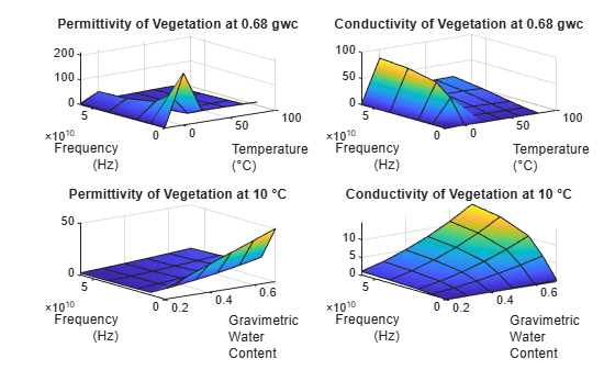
Compare the real relative permittivity and conductivity for varying values of frequency, temperature, and gravimetric water content.

Specify frequency, temperature, and gravimetric water content values using vectors. Create grids from the values by repeating the vectors.

fc0 = [0.1 10 20 40 60]*1e9;
temp0 = -20:20:80;
gwc0 = 0.2:0.1:0.7;

fc = repmat(fc0,6,1);
temp = repmat(temp0',1,5);
gwc = repmat(gwc0',1,5);

For each frequency and temperature value, calculate the permittivity and conductivity of vegetation. Use a gravimetric water content value of 0.68. Apply the earthSurfacePermittivity function to each element of the gridded inputs by using the arrayfun function.

[epsilon_veg_gwc,sigma_veg_gwc] = arrayfun(@(x,y) ...
    earthSurfacePermittivity("vegetation",x,y,0.68),fc,temp);

For each frequency and gravimetric water content value, calculate the permittivity and conductivity of vegetation. Use a temperature value of 10 °C.

[epsilon_veg_tmp,sigma_veg_tmp] = arrayfun(@(x,z) ...
    earthSurfacePermittivity("vegetation",x,10,z),fc,gwc);

Display the results using multiple surface plots. Organize the plots using a tiled chart layout.

figure
tiledlayout(2,2)

nexttile
surf(temp,fc,epsilon_veg_gwc,FaceColor="interp")
title("Permittivity of Vegetation at 0.68 gwc")
xlabel(["Temperature","(°C)"])
ylabel(["Frequency","(Hz)"])

nexttile
surf(temp,fc,sigma_veg_gwc,"FaceColor","interp")
title("Conductivity of Vegetation at 0.68 gwc")
xlabel(["Temperature","(°C)"])
ylabel(["Frequency","(Hz)"])

nexttile
surf(gwc,fc,epsilon_veg_tmp,"FaceColor","interp")
title("Permittivity of Vegetation at 10 °C")
xlabel(["Gravimetric","Water","Content"])
ylabel(["Frequency","(Hz)"])

nexttile
surf(gwc,fc,sigma_veg_tmp,"FaceColor","interp")
title("Conductivity of Vegetation at 10 °C")
xlabel(["Gravimetric","Water","Content"])
ylabel(["Frequency","(Hz)"])

Input Arguments

General

fc — Carrier frequency in Hz

numeric scalar

Carrier frequency in Hz, specified as a numeric scalar. For most surfaces, this value must be in the range (0, 10¹²]. For multi-year ice, dry snow, and wet snow, this value must be in the range (0, 10¹¹].

Data Types: double

temp — Temperature in °C

numeric scalar

Temperature in °C, specified as a numeric scalar. This table indicates the valid temperature limits for each surface.

Surface	Valid Temperature Limits (°C)
Pure water	[–4, 40]
Sea water	[–4, 40]
Pure ice	[–60, 0]
Wet ice	N/A, but the function assumes 0
Multi-year ice	[–30, –2]
Dry snow	[–60, 0]
Wet snow	[–60, 0]
Soil	Any numeric scalar
vegetation	Greater than or equal to –20

Data Types: double

Water

salinity — Salinity of sea water in g/kg

numeric scalar in range [0, 40]

Salinity of the sea water in g/kg, specified as a numeric scalar in the range [0, 40].

Data Types: double

Ice

liqfrac — Liquid water volume fraction of wet ice

numeric scalar in range [0, 1]

Liquid water volume fraction of the wet ice, specified as a numeric scalar in the range [0, 1].

Data Types: double

avf — Air volume fraction of multi-year ice

numeric scalar in range [0, 1]

Air volume fraction of the multi-year ice, specified as a numeric scalar in the range [0, 1].

Data Types: double

Snow

dsd — Dry snow density of snow in g/cm³

nonnegative numeric scalar

Dry snow density of the snow in g/cm³, specified as a nonnegative numeric scalar.

Data Types: double

lwc — Liquid water volume fraction of wet snow

numeric scalar in range [0, 1]

Liquid water volume fraction of the wet snow, specified as a numeric scalar in the range [0, 1].

Data Types: double

Soil

sandpercent — Sand percentage of soil by volume

numeric scalar in range [0, 100]

Sand percentage of the soil by volume, specified as a numeric scalar in the range [0, 100]. The sum of sandpercent and claypercent must be less than or equal to 100.

Data Types: double

claypercent — Clay percentage of soil by volume

numeric scalar in range [0, 100]

Clay percentage of the soil by volume, specified as a numeric scalar in the range [0, 100]. The sum of sandpercent and claypercent must be less than or equal to 100.

Data Types: double

sg — Specific gravity of soil

nonnegative scalar

Specific gravity of the soil, specified as a nonnegative scalar. The specific gravity is the mass density of the soil sample divided by the mass density of the amount of water in the soil sample.

Data Types: double

vwc — Volumetric water content of soil

numeric scalar in range [0, 1]

Volumetric water content of the soil, specified as a numeric scalar in the range [0, 1]. For more information about volumetric water content, see Soil Contents.

Data Types: double

bulkdensity — Bulk density of soil in g/cm³

nonnegative scalar

Bulk density of the soil in g/cm³, specified as a nonnegative scalar. For more information about bulk density, see Soil Contents.

Data Types: double

Vegetation

gwc — Gravimetric water content of vegetation

numeric scalar in range [0, 0.7]

Gravimetric water content of the vegetation, specified as a numeric scalar in the range [0, 0.7]. For more information about gravimetric water content, see Soil Contents.

Data Types: double

Output Arguments

epsilon — Real relative permittivity

numeric scalar

Real relative permittivity of the earth surface, returned as a numeric scalar.

sigma — Conductivity in S/m

nonnegative scalar

Conductivity of the earth surface in S/m, returned as a nonnegative scalar.

complexepsilon — Complex relative permittivity

complex scalar

Complex relative permittivity of the earth surface, returned as a complex scalar.

More About

ITU Terrain Materials

ITU-R P.527-5 through ITU-R P.527-6 [1] present methods and equations to calculate complex relative permittivity at carrier frequencies up to 1,000 GHz for common earth surface materials. The earthSurfacePermittivity function supports these materials:

• Pure water

• Sea water

• Pure ice

• Wet ice

• Multi-year ice (since R2024a)

• Dry snow (since R2024a)

• Wet snow (since R2024a)

• Soil

• Vegetation

Soil Contents

ITU-R P.527-6 uses these metrics to quantify soil:

• The percentages of sand, clay, and silt by volume in the soil. Specify the percentages of sand and clay by volume using the sandpercent and claypercent arguments. The function calculates the percent of silt by volume by subtracting sandpercent and claypercent from 100.

• The specific gravity of the soil, which is the mass density of the soil divided by the mass density of the water. Specify the specific gravity using the sg argument.

• The volumetric water content of the soil, which is the volume of liquid water per volume of soil. Specify the volumetric water content using the vwc argument.

• The bulk density of the soil, which is the ratio of the dry soil weight to the volume of the soil sample. Specify the bulk density using the bulkdensity argument. When you do not specify the bulkdensity argument, the function derives bulkdensity using equation (57) of ITU-R P.527-6:

  bulkdensity = 1.07256 + 0.078886 ln(sandpercent) + 0.038753 ln(claypercent) + 0.032732 ln(100-(sandpercent + claypercent))

This table repeats the contents of Table 2 from ITU-R P.527-6, which shows typical metrics for sandy loam, loam, silty loam, and silty clay soil types.

Quality	Sandy Loam	Loam	Silty Loam	Silty Clay
Percentage of sand	51.52	41.96	30.63	5.02
Percentage of clay	13.42	8.53	13.48	47.38
Percentage of silt	35.06	49.51	55.89	47.60
Specific gravity (ρs)	2.66	2.70	2.59	2.56
Bulk density (ρb) in g/cm3	1.6006	1.5781	1.5750	1.4758

References

[1] International Telecommunications Union Radiocommunication Sector. Electrical Characteristics of the Surface of the Earth. Recommendation P.527. ITU-R, approved September 27, 2021. https://www.itu.int/rec/R-REC-P.527/en.

Extended Capabilities

C/C++ Code Generation
Generate C and C++ code using MATLAB® Coder™.

Version History

Introduced in R2020a

R2024a: Model surfaces using updated ITU recommendations

The earthSurfacePermittivity function models surfaces using the methods and equations in ITU-R P.527-5 through ITU-R P.527-6 [1].

In addition:

• The valid temperature limits for pure water and sea water are now in the range [–4, 40].

• The valid temperature limits for pure ice are now in the range [–60, 0].

• The valid salinity limits for sea water are now in the range [0, 40].

• The "dry-ice" input is now "pure-ice". To update your code, replace uses of "dry-ice" with "pure-ice". There are no plans to remove the "dry-ice" input.

• When you specify "soil" as input and do not specify a bulk density, the function can return different values in R2024a compared to previous releases.

R2024a: Model multi-year ice, dry snow, and wet snow surfaces

Calculate the real relative permittivity, conductivity, and complex relative permittivity of multi-year ice, dry now, and wet snow surfaces.