step
System object: phased.RangeResponse
Namespace: phased
Range response
Syntax
Description
Note
Instead of using the step method to perform
the operation defined by the System object™, you can call the object
with arguments, as if it were a function. For example, y
= step(obj,x) and y = obj(x) perform
equivalent operations.
[ computes
the range response, resp,rnggrid]
= step(response,x)resp, for the input signal, x,
and the range values, rnggrid, corresponding to the
response. This syntax applies when you set RangeMethod to 'FFT' and DechirpInput to false.
This syntax assumes that the input signal has already been dechirped.
This syntax is most commonly used with FMCW signals.
[ computes
the range response of the input signal, resp,rnggrid]
= step(response,x,xref)x using
the reference signal, xref. This syntax applies
when you set RangeMethod to 'FFT' and DechirpInput to true.
Often, the reference signal is the transmitted signal. This syntax
assumes that the input signal has not been dechirped. This syntax
is most commonly used with FMCW signals.
Note
The object performs an initialization the first time the object is executed. This
initialization locks nontunable properties
and input specifications, such as dimensions, complexity, and data type of the input data.
If you change a nontunable property or an input specification, the System object issues an error. To change nontunable properties or inputs, you must first
call the release method to unlock the object.
Input Arguments
Output Arguments
Examples
Compute the radar range response of three targets by using the phased.RangeResponse System object™. The transmitter and receiver are collocated isotropic antenna elements forming a monostatic radar system. The transmitted signal is a linear FM waveform with a pulse repetition interval of 7.0 μs and a duty cycle of 2%. The operating frequency is 77 GHz and the sample rate is 150 MHz.
fs = 150e6;
c = physconst('LightSpeed');
fc = 77e9;
pri = 7e-6;
prf = 1/pri;
Set up the scenario parameters. The radar transmitter and receiver are stationary and located at the origin. The targets are 500, 530, and 750 meters from the radars on the x-axis. The targets move along the x-axis at speeds of −60, 20, and 40 m/s. All three targets have a nonfluctuating radar cross-section (RCS) of 10 dB.
Create the target and radar platforms.
Numtgts = 3;
tgtpos = zeros(Numtgts);
tgtpos(1,:) = [500 530 750];
tgtvel = zeros(3,Numtgts);
tgtvel(1,:) = [-60 20 40];
tgtrcs = db2pow(10)*[1 1 1];
tgtmotion = phased.Platform(tgtpos,tgtvel);
target = phased.RadarTarget('PropagationSpeed',c,'OperatingFrequency',fc, ...
    'MeanRCS',tgtrcs);
radarpos = [0;0;0];
radarvel = [0;0;0];
radarmotion = phased.Platform(radarpos,radarvel);
Create the transmitter and receiver antennas.
txantenna = phased.IsotropicAntennaElement;
rxantenna = clone(txantenna);
Set up the transmitter-end signal processing. Create an upsweep linear FM signal with a bandwidth of half the sample rate. Find the length of the pri in samples and then estimate the rms bandwidth and range resolution.
bw = fs/2;
waveform = phased.LinearFMWaveform('SampleRate',fs, ...
    'PRF',prf,'OutputFormat','Pulses','NumPulses',1,'SweepBandwidth',fs/2, ...
    'DurationSpecification','Duty cycle','DutyCycle',0.02);
sig = waveform();
Nr = length(sig);
bwrms = bandwidth(waveform)/sqrt(12);
rngrms = c/bwrms;
Set up the transmitter and radiator System object properties. The peak output power is 10 W and the transmitter gain is 36 dB.
peakpower = 10;
txgain = 36.0;
transmitter = phased.Transmitter( ...
    'PeakPower',peakpower, ...
    'Gain',txgain, ...
    'InUseOutputPort',true);
radiator = phased.Radiator( ...
    'Sensor',txantenna, ...
    'PropagationSpeed',c, ...
    'OperatingFrequency',fc);
Create a free-space propagation channel in two-way propagation mode.
channel = phased.FreeSpace( ...
    'SampleRate',fs, ...
    'PropagationSpeed',c, ...
    'OperatingFrequency',fc, ...
    'TwoWayPropagation',true);
Set up the receiver-end processing. The receiver gain is 42 dB and noise figure is 10.
collector = phased.Collector( ...
    'Sensor',rxantenna, ...
    'PropagationSpeed',c, ...
    'OperatingFrequency',fc);
rxgain = 42.0;
noisefig = 10;
receiver = phased.ReceiverPreamp( ...
    'SampleRate',fs, ...
    'Gain',rxgain, ...
    'NoiseFigure',noisefig);
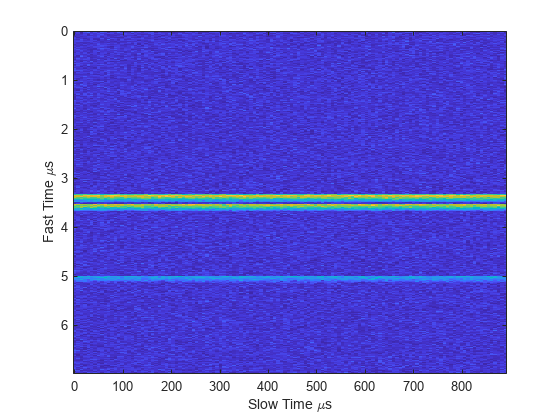
Loop over 128 pulses to build a data cube. For each step of the loop, move the target and propagate the signal. Then put the received signal into the data cube. The data cube contains the received signal per pulse. Ordinarily, a data cube has three dimensions, where last dimension corresponds to antennas or beams. Because only one sensor is used in this example, the cube has only two dimensions.
The processing steps are:
Move the radar and targets.
Transmit a waveform.
Propagate the waveform signal to the target.
Reflect the signal from the target.
Propagate the waveform back to the radar. Two-way propagation mode enables you to combine the returned propagation with the outbound propagation.
Receive the signal at the radar.
Load the signal into the data cube.
Np = 128;
cube = zeros(Nr,Np);
for n = 1:Np
    [sensorpos,sensorvel] = radarmotion(pri);
    [tgtpos,tgtvel] = tgtmotion(pri);
    [tgtrng,tgtang] = rangeangle(tgtpos,sensorpos);
    sig = waveform();
    [txsig,txstatus] = transmitter(sig);
    txsig = radiator(txsig,tgtang);
    txsig = channel(txsig,sensorpos,tgtpos,sensorvel,tgtvel);
    tgtsig = target(txsig);
    rxcol = collector(tgtsig,tgtang);
    rxsig = receiver(rxcol);
    cube(:,n) = rxsig;
end
Display the image of the data cube containing signals per pulse.
imagesc([0:(Np-1)]*pri*1e6,[0:(Nr-1)]/fs*1e6,abs(cube))
xlabel('Slow Time {\mu}s')
ylabel('Fast Time {\mu}s')
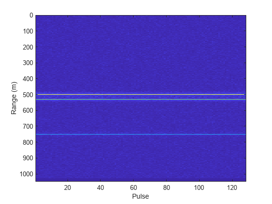
Create a phased.RangeResponse System object in matched filter mode. Then, display the range response image for the 128 pulses. The image shows range vertically and pulse number horizontally.
matchingcoeff = getMatchedFilter(waveform);
ndop = 128;
rangeresp = phased.RangeResponse('SampleRate',fs,'PropagationSpeed',c);
[resp,rnggrid] = rangeresp(cube,matchingcoeff);
imagesc([1:Np],rnggrid,abs(resp))
xlabel('Pulse')
ylabel('Range (m)')
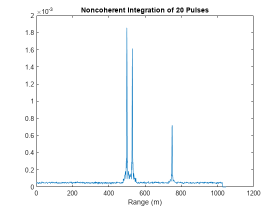
Integrate 20 pulses noncoherently.
intpulse = pulsint(resp(:,1:20),'noncoherent');
plot(rnggrid,abs(intpulse))
xlabel('Range (m)')
title('Noncoherent Integration of 20 Pulses')
Version History
Introduced in R2017a