phased.GSCBeamformer
Generalized sidelobe canceler beamformer
Description
The phased.GSCBeamformer
System object™ implements a generalized sidelobe cancellation (GSC) beamformer. A GSC
beamformer splits the incoming signals into two channels. One channel goes through a
conventional beamformer path and the second goes into a sidelobe canceling path. The algorithm
first pre-steers the array to the beamforming direction and then adaptively chooses filter
weights to minimize power at the output of the sidelobe canceling path. The algorithm uses
least mean squares (LMS) to compute the adaptive weights. The final beamformed signal is the
difference between the outputs of the two paths.
To compute the beamformed signal:
Create the
phased.GSCBeamformerobject and set its properties.Call the object with arguments, as if it were a function.
To learn more about how System objects work, see What Are System Objects?
Creation
Description
beamformer = phased.GSCBeamformerbeamformer, with default property values.
beamformer = phased.GSCBeamformer(Name,Value)beamformer, with each specified
property Name set to the specified Value. You can specify additional name-value pair
arguments in any order as
(Name1,Value1,...,NameN,ValueN).
Enclose each property name in single quotes.
Example: beamformer =
phased.GSCBeamformer('SensorArray',phased.ULA('NumElements',20),'SampleRate',300e3)
sets the sensor array to a uniform linear array (ULA) with default ULA property values
except for the number of elements. The beamformer has a sample rate of 300
kHz.
Properties
Usage
Description
Input Arguments
Output Arguments
Object Functions
To use an object function, specify the
System object as the first input argument. For
example, to release system resources of a System object named obj, use
this syntax:
release(obj)
Examples
Create a GSC beamformer for a 11-element acoustic array in air. A chirp signal is incident on the array at in azimuth and in elevation. Compare the GSC beamformed signal to a Frost beamformed signal. The signal propagation speed is 340 m/s and the sample rate is 8 kHz.
Create the microphone and array System objects. The array element spacing is one-half wavelength. Set the signal frequency to the one-half the Nyquist frequency.
c = 340.0;
fs = 8.0e3;
fc = fs/2;
lam = c/fc;
transducer = phased.OmnidirectionalMicrophoneElement('FrequencyRange',[20 20000]);
array = phased.ULA('Element',transducer,'NumElements',11,'ElementSpacing',lam/2);
Simulate a chirp signal with a 500 Hz bandwidth.
t = 0:1/fs:.5;
signal = chirp(t,0,0.5,500);
Create an incident wave arriving at the array. Add gaussian noise to the wave.
collector = phased.WidebandCollector('Sensor',array,'PropagationSpeed',c, ...
    'SampleRate',fs,'ModulatedInput',false,'NumSubbands',512);
incidentAngle = [-50;0];
signal = collector(signal.',incidentAngle);
noise = 0.5*randn(size(signal));
recsignal = signal + noise;
Perform Frost beamforming at the actual incident angle.
frostbeamformer = phased.FrostBeamformer('SensorArray',array,'PropagationSpeed', ...
    c,'SampleRate',fs,'Direction',incidentAngle,'FilterLength',15);
yfrost = frostbeamformer(recsignal);
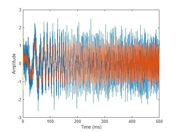
Perform GSC beamforming and plot the beamformer output against the Frost beamformer output. Also plot the nonbeamformed signal arriving at the middle element of the array.
gscbeamformer = phased.GSCBeamformer('SensorArray',array, ...
    'PropagationSpeed',c,'SampleRate',fs,'Direction',incidentAngle, ...
    'FilterLength',15);
ygsc = gscbeamformer(recsignal);
plot(t*1000,recsignal(:,6),t*1000,yfrost,t,ygsc)
xlabel('Time (ms)')
ylabel('Amplitude')
Zoom in on a small portion of the output.
idx = 1000:1300;
plot(t(idx)*1000,recsignal(idx,6),t(idx)*1000,yfrost(idx),t(idx)*1000,ygsc(idx))
xlabel('Time (ms)')
legend('Received signal','Frost beamformed signal','GSC beamformed signal')

Create a GSC beamformer for an 11-element acoustic array in air. A chirp signal is incident on the array at in azimuth and in elevation. Compute the beamformed signal in the direction of the incident wave and in another direction. Compare the two beamformed outputs. The signal propagation speed is 340 m/s and the sample rate is 8 kHz. Create the microphone and array System objects. The array element spacing is one-half wavelength. Set the signal frequency to the one-half the Nyquist frequency.
c = 340.0;
fs = 8.0e3;
fc = fs/2;
lam = c/fc;
transducer = phased.OmnidirectionalMicrophoneElement('FrequencyRange',[20 20000]);
array = phased.ULA('Element',transducer,'NumElements',11,'ElementSpacing',lam/2);
Simulate a chirp signal with a 500 Hz bandwidth.
t = 0:1/fs:0.5;
signal = chirp(t,0,0.5,500);
Create an incident wavefield hitting the array.
collector = phased.WidebandCollector('Sensor',array,'PropagationSpeed',c, ...
    'SampleRate',fs,'ModulatedInput',false,'NumSubbands',512);
incidentAngle = [-50;0];
signal = collector(signal.',incidentAngle);
noise = 0.1*randn(size(signal));
recsignal = signal + noise;
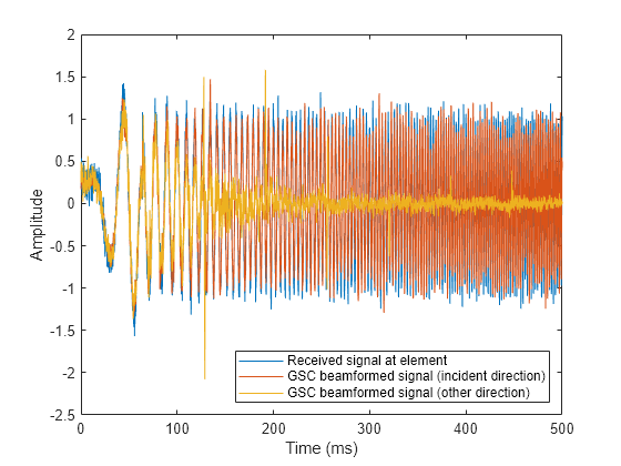
Perform GSC beamforming and plot the beamformer outputs. Also plot the nonbeamformed signal arriving at the middle element of the array.
gscbeamformer = phased.GSCBeamformer('SensorArray',array, ...
    'PropagationSpeed',c,'SampleRate',fs,'DirectionSource','Input port', ...
    'FilterLength',5);
ygsci = gscbeamformer(recsignal,incidentAngle);
ygsco = gscbeamformer(recsignal,[20;30]);
plot(t*1000,recsignal(:,6),t*1000,ygsci,t*1000,ygsco)
xlabel('Time (ms)')
ylabel('Amplitude')
legend('Received signal at element','GSC beamformed signal (incident direction)', ...
    'GSC beamformed signal (other direction)','Location','southeast')
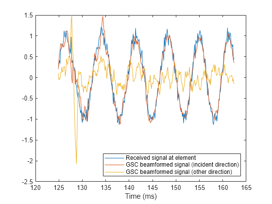
Zoom in on a small portion of the output.
idx = 1000:1300;
plot(t(idx)*1000,recsignal(idx,6),t(idx)*1000,ygsci(idx),t(idx)*1000,ygsco(idx))
xlabel('Time (ms)')
legend('Received signal at element','GSC beamformed signal (incident direction)', ...
    'GSC beamformed signal (other direction)','Location','southeast')
Algorithms
The generalized sidelobe canceler (GSC) is an efficient implementation of a linear constraint minimum variance (LCMV) beamformer. LCMV beamforming minimizes the output power of an array while preserving the power in one or more specified directions. This type of beamformer is called a constrained beamformer. You can compute exact weights for the constrained beamformer but the computation is costly when the number of elements is large. The computation requires the inversion of a large spatial covariance matrix. The GSC formulation converts the adaptive constrained optimization LCMV problem into an adaptive unconstrained problem, which simplifies the implementation.
In the GSC algorithm, incoming sensor data is split into two signal paths as shown in the block diagram. The upper path is a conventional beamformer. The lower path is an adaptive unconstrained beamformer whose purpose is to minimize the GSC output power. The GSC algorithm consists of these steps:
Presteer the element sensor data by time-shifting the incoming signals. Presteering time-aligns all sensor element signals. The time shifts depend on the arrival angle of the signal.
Pass the presteered signals through the upper path into a conventional beamformer with fixed weights, wconv.
Also pass the presteered signals through the lower path into the blocking matrix, B. The blocking matrix is orthogonal to the signal and removes the signal from the lower path.
Filter the lower path signals through a bank of FIR filters. The FilterLength property sets the length of the filters. The filter coefficients are the adaptive filter weights, wad.
Compute the difference between the upper and lower signal paths. This difference is the beamformed GSC output.
Feed the beamformed output back into the filter. The filter adapts its weights using a least mean-square (LMS) algorithm. The actual adaptive LMS step size is equal to the value of the LMSStepSize property divided by the total signal power.

For more information, see [1].
References
[1] Griffiths, L. J., and Charles W. Jim. "An alternative approach to linearly constrained adaptive beamforming." IEEE Transactions on Antennas and Propagation, 30.1 (1982): 27-34.
[2] Van Trees, H. Optimum Array Processing. New York: Wiley-Interscience, 2002.
[3] Johnson, D.H., and Dan E. Dudgeon, Array Signal Processing, Englewood Cliffs: Prentice-Hall, 1993.
Extended Capabilities
Version History
Introduced in R2016b