evaluateTemperatureGradient
Evaluate temperature gradient of thermal solution at arbitrary spatial locations
Syntax
Description
[
returns the interpolated values of temperature gradients of the thermal model
solution gradTx,gradTy]
= evaluateTemperatureGradient(thermalresults,xq,yq)thermalresults at the 2-D points specified in
xq and yq. This syntax is valid for both
the steady-state and transient thermal models.
[___] = evaluateTemperatureGradient(
returns the interpolated values of the temperature gradients at the points specified
in thermalresults,querypoints)querypoints. This syntax is valid for both the steady-state
and transient thermal models.
[___] = evaluateTemperatureGradient(___,
returns the interpolated values of the temperature gradients for the time-dependent
equation at times iT)iT. Specify iT after the
input arguments in any of the previous syntaxes.
The first dimension of gradTx, gradTy,
and, in 3-D case, gradTz corresponds to query points. The
second dimension corresponds to time-steps iT.
Examples
For a 2-D steady-state thermal problem, evaluate temperature gradients at the nodal locations and at the points specified by x and y coordinates.
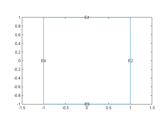
Create and plot a square geometry.
R1 = [3,4,-1,1,1,-1,1,1,-1,-1]';
g = decsg(R1,'R1',('R1')');
pdegplot(g,EdgeLabels="on")
xlim([-1.1 1.1])
ylim([-1.1 1.1])
Create an femodel object for steady-state thermal analysis and include the geometry into the model.
model = femodel(AnalysisType="thermalSteady", ...
                Geometry=g);
Assuming that this geometry represents an iron plate, the thermal conductivity is .
model.MaterialProperties = ...
    materialProperties(ThermalConductivity=79.5);
Apply a constant temperature of 300 K to the bottom of the plate (edge 3).
model.EdgeBC(3) = edgeBC(Temperature=300);
Apply convection on the two sides of the plate (edges 2 and 4).
model.EdgeLoad([2 4]) = ...
    edgeLoad(ConvectionCoefficient=25,...
             AmbientTemperature=50);
Mesh the geometry and solve the problem.
model = generateMesh(model);
R = solve(model)
R =
  SteadyStateThermalResults with properties:

    Temperature: [1529×1 double]
     XGradients: [1529×1 double]
     YGradients: [1529×1 double]
     ZGradients: []
           Mesh: [1×1 FEMesh]
The solver finds the temperatures and temperature gradients at the nodal locations. To access these values, use R.Temperature, R.XGradients, and so on. For example, plot the temperature gradients at nodal locations.
figure
pdeplot(R.Mesh,FlowData=[R.XGradients R.YGradients]);
axis equal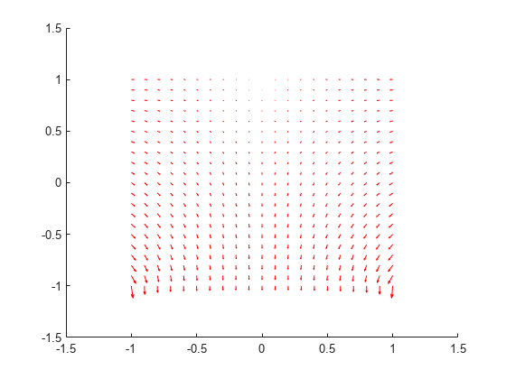
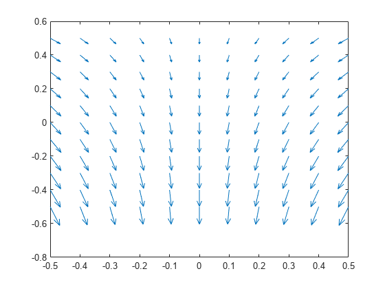
Create a grid specified by x and y coordinates, and evaluate temperature gradients to the grid.
v = linspace(-0.5,0.5,11);
[X,Y] = meshgrid(v);

[gradTx,gradTy] = ...
evaluateTemperatureGradient(R,X,Y);
Reshape the gradTx and gradTy vectors, and plot the resulting temperature gradients.
gradTx = reshape(gradTx,size(X));
gradTy = reshape(gradTy,size(Y));
figure
quiver(X,Y,gradTx,gradTy)
axis equal
Alternatively, you can specify the grid by using a matrix of query points.
querypoints = [X(:) Y(:)]';
[gradTx,gradTy] = ...
evaluateTemperatureGradient(R,querypoints);

gradTx = reshape(gradTx,size(X));
gradTy = reshape(gradTy,size(Y));
figure
quiver(X,Y,gradTx,gradTy)
axis equal
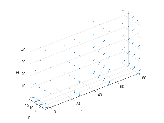
For a 3-D steady-state thermal problem, evaluate temperature gradients at the nodal locations and at the points specified by x, y, and z coordinates.
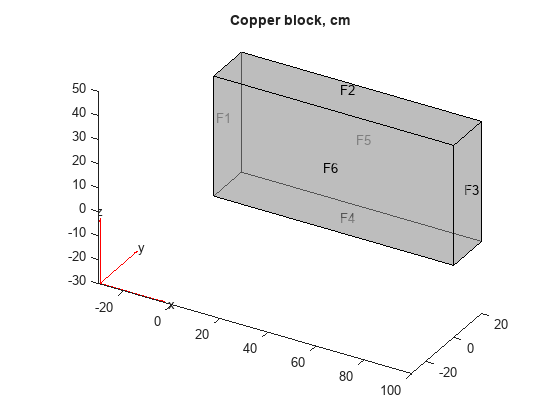
Create an femodel object for steady-state thermal analysis and include a block geometry into the model.
model = femodel(AnalysisType="thermalSteady", ...
                Geometry="Block.stl");
Plot the geometry.
pdegplot(model.Geometry,FaceLabels="on",FaceAlpha=0.5)
title("Copper block, cm")
Assuming that this is a copper block, the thermal conductivity of the block is approximately .
model.MaterialProperties = ...
    materialProperties(ThermalConductivity=4);
Apply a constant temperature of 373 K to the left side of the block (edge 1) and a constant temperature of 573 K to the right side of the block.
model.FaceBC(1) = faceBC(Temperature=373);
model.FaceBC(3) = faceBC(Temperature=573);
Apply a heat flux boundary condition to the bottom of the block.
model.FaceLoad(4) = faceLoad(Heat=-20);
Mesh the geometry and solve the problem.
model = generateMesh(model);
R = solve(model)
R =
  SteadyStateThermalResults with properties:

    Temperature: [12822×1 double]
     XGradients: [12822×1 double]
     YGradients: [12822×1 double]
     ZGradients: [12822×1 double]
           Mesh: [1×1 FEMesh]
The solver finds the values of temperatures and temperature gradients at the nodal locations. To access these values, use R.Temperature, R.XGradients, and so on.
Create a grid specified by x, y, and z coordinates, and evaluate temperature gradients to the grid.
[X,Y,Z] = meshgrid(1:26:100,1:6:20,1:11:50);

[gradTx,gradTy,gradTz] = ...
evaluateTemperatureGradient(R,X,Y,Z);
Reshape the gradTx, gradTy, and gradTz vectors, and plot the resulting temperature gradients.
gradTx = reshape(gradTx,size(X));
gradTy = reshape(gradTy,size(Y));
gradTz = reshape(gradTz,size(Z));

figure
quiver3(X,Y,Z,gradTx,gradTy,gradTz)
axis equal
xlabel("x")
ylabel("y")
zlabel("z")

Alternatively, you can specify the grid by using a matrix of query points.
querypoints = [X(:) Y(:) Z(:)]';
[gradTx,gradTy,gradTz] = ...
evaluateTemperatureGradient(R,querypoints);

gradTx = reshape(gradTx,size(X));
gradTy = reshape(gradTy,size(Y));
gradTz = reshape(gradTz,size(Z));

figure
quiver3(X,Y,Z,gradTx,gradTy,gradTz)
axis equal
xlabel("x")
ylabel("y")
zlabel("z")
Solve a 2-D transient heat transfer problem on a square domain and compute temperature gradients at the convective boundary.
Create an femodel object for transient thermal analysis and include a square geometry into the model.
model = femodel(AnalysisType="thermalTransient", ...
                Geometry=@squareg);
Plot the geometry.
pdegplot(model.Geometry,EdgeLabels="on")
xlim([-1.1 1.1])
ylim([-1.1 1.1])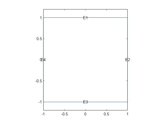
Assign the following thermal properties: thermal conductivity is , mass density is , and specific heat is .
model.MaterialProperties = ...
    materialProperties(ThermalConductivity=100,...
                       MassDensity=7800,...
                       SpecificHeat=500);
Apply the convection boundary condition on the right edge.
model.EdgeLoad(2) = ...
    edgeLoad(ConvectionCoefficient=5000,...
             AmbientTemperature=25);
Set the initial conditions: uniform room temperature across domain and higher temperature on the left edge.
model.FaceIC = faceIC(Temperature=25);
model.EdgeIC(4) = edgeIC(Temperature=100);
Generate a mesh and solve the problem using 0:1000:200000 as a vector of times.
model = generateMesh(model);
tlist = 0:1000:200000;
R = solve(model,tlist);
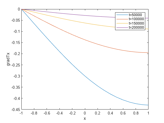
Define a line at convection boundary and compute temperature gradients across that line.
X = -1:0.1:1;
Y = ones(size(X));

[gradTx,gradTy] = ...
    evaluateTemperatureGradient(R,X,Y,1:length(tlist));
Plot the interpolated gradient component gradTx along the x axis for the following values from the time interval tlist.
figure
t = [51:50:201];
for i = t
  p(i) = plot(X,gradTx(:,i), ...
      DisplayName=strcat("t=",num2str(tlist(i))));
  hold on
end
legend(p(t))
xlabel("x")
ylabel("gradTx")
Input Arguments
Output Arguments
Version History
Introduced in R2017a