Diversify Portfolios Using Optimization Toolbox
This example shows three techniques of asset diversification in a portfolio. The purpose of asset diversification is to balance the exposure of the portfolio to any given asset in order to reduce volatility over a period of time. Given the sensitivity of the minimum variance portfolio to the estimation of the covariance matrix, some practitioners have added diversification techniques to the portfolio selection with the hope of minimizing risk measures other than the variance measures such as turnover, maximum drawdown, and so on.
This example presents these common diversification techniques:
Equally weighted (EW) portfolio
Equal risk contribution (ERC)
Most diversified portfolio (MDP)
Additionally, this example demonstrates penalty methods that can be used to achieve different degrees of diversification. In those methods, a penalty term is added to the objective function to balance the level of variance reduction and the diversification of the portfolio.
Retrieve Market Data and Define Mean-Variance Portfolio
Begin by loading and computing the expected returns and their covariance matrix.
% Load data
load("port5.mat");
% Store returns and covariance
mu = mean_return;
Sigma = Correlation .* (stdDev_return * stdDev_return');
Define a mean-variance portfolio using a Portfolio (Financial Toolbox) object with default constraints to create a fully invested, long-only portfolio.
% Create a mean-variance Portfolio object with default constraints
p = Portfolio(AssetMean=mu,AssetCovar=Sigma);
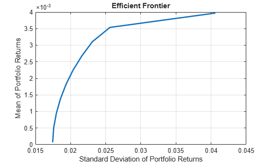
p = setDefaultConstraints(p);One of the many features of the Portfolio (Financial Toolbox) object is that it can obtain the efficient frontier of the portfolio problem. The efficient frontier is computed by solving a series of optimization problems for which the return level of the portfolio, , is modified to obtain different points on the efficient frontier. These problems are defined as
The advantage of using the Portfolio (Financial Toolbox) object to compute the efficient frontier is that it is obtained without having to manually formulate and solve the multiple optimization problems shown above.
plotFrontier(p);
The Portfolio (Financial Toolbox) object can also compute the weights associated to the minimum variance portfolio, which is defined by the following problem.
The minimum variance weights is considered the benchmark against which all the weights of the diversification strategies are compared.
wMinVar = estimateFrontierLimits(p,"min");The Portfolio (Financial Toolbox) object can compute the minimum variance portfolio. However, the diversification strategies add modifications to the objective function of the portfolio problem that are not supported by the Portfolio (Financial Toolbox) object for MATLAB® versions before R2022b. For earlier versions, you must use Optimization Toolbox™ to solve the following problems. To learn more about the problems that can be solved by the Portfolio (Financial Toolbox) object, see When to Use Portfolio Objects Over Optimization Toolbox (Financial Toolbox).
Specify Diversification Techniques
This section presents the three diversification methods. Each of the three diversification methods is associated with a diversification measure and that diversification measure is used to define a penalty term to achieve different diversification levels. The diversification, obtained by adding the penalty term to the objective function, ranges from the behavior achieved by the minimum variance portfolio to the behavior of the EW, ECR, and MDP, respectively.
Start by initializing an optimproblem object and define its constraints. All the following portfolio problems have the same constraints and only the objective function changes. Therefore, the following optimproblem can be reused while the objective function is redefined accordingly.
% Define an optimization problem to adjust portfolio diversification
diverseProb = optimproblem(ObjectiveSense="minimize");
The default portfolio has only one equality constraint and a lower bound for the assets weights. The weights must be nonnegative and they must sum to 1. The feasible set is represented as:
% Variables
nX = p.NumAssets;
% Portfolio weights [nX-by-1 vector]
x = optimvar("x",nX,1,LowerBound=0); % x >= 0 (long-only portfolio)

% Equality constraint
% Sum of weights equal to one
diverseProb.Constraints.fullyInvested = sum(x) == 1;
The first part of the example shows how to compute the minimum variance portfolio using the Portfolio (Financial Toolbox) object. However, the minimum variance weights can also be obtained with the following piece of code that represents the minimum variance problem:
% Minimize variance
diverseProb.Objective = x'*p.AssetCovar*x;
% Solution of minimum variance portfolio
opts = optimoptions("quadprog",Display="none"); % No output display
[wMinVar2,fMinVar,c,d,e] = solve(diverseProb,Options=opts);
The solution above and the one obtained by the Portfolio (Financial Toolbox) object are not exactly the same.
norm(wMinVar-wMinVar2.x,inf)
ans =
0.0032
This result happens because the minimum variance problem is badly scaled given the size of the eigenvalues of the covariance matrix. If the objective function is rescaled by a large constant (for example, 1e4), then both solutions coincide within numerical accuracy. This capability is another advantage of using the Portfolio (Financial Toolbox) object. The Portfolio (Financial Toolbox) object rescales the problem by default to resolve numerical issues, so it obtains a portfolio with smaller variance than the one obtained without scaling the problem.
Since the purpose of the example is to show the different diversification strategies, this example proceeds without rescaling the optimization problems. However, keep in mind that the variance term () can be rescaled in any of the following problems.
Equally Weighted (EW) Portfolio
One of the diversification measures is the Herfindahl-Hirschman (HH) index defined as:
This index is minimized when the portfolio is equally weighted. The portfolios obtained from using this index as a penalty have weights that satisfy the portfolio constraints and that are more evenly weighted.
The portfolio that minimizes the HH index is . Since the constraints in are the default constraints, the solution of this problem is the EW portfolio. If had extra constraints, the solution would be the portfolio that satisfies all the constraints and, at the same time, keeps the weights as equal as possible.
% Maximize the HH diversification (by minimizing the HH index)
diverseProb.Objective = x'*x;
% Solution that minimizes the HH index
[wHH,fHH] = solve(diverseProb,Options=opts);
The portfolio that minimizes the variance with the HH penalty is .
% HH penalty parameter
lambdaHH = 1e-2;
% Variance + Herfindahl-Hirschman (HH) index
diverseProb.Objective = x'*p.AssetCovar*x + lambdaHH*(x'*x);
% Solution that accounts for risk and HH diversification
[wHHMix,fHHMix] = solve(diverseProb,Options=opts);
Plot the weights distribution for the minimum variance portfolio, the equal weight portfolio, and the penalized strategy.
% Plot different strategies
plotAssetAllocationChanges(wMinVar,wHHMix.x,wHH.x)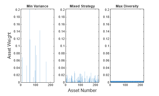
This plot shows how the penalized strategy returns weights that are between the minimum variance portfolio and the EW portfolio. In fact, choosing returns the minimum variance solution, and as the solution approaches the EW portfolio.
Most Diversified Portfolio (MDP)
The diversification index associated to the most diversified portfolio (MDP) is defined as
where represents the standard deviation of asset .
The MDP is the portfolio that maximizes the diversification ratio:
The diversification ratio is equal to 1 if the portfolio is fully invested in one asset or if all assets are perfectly correlated. For all other cases, . If , there is no diversification, so the goal is to find the portfolio that maximizes :
Instead of solving the nonlinear, nonconvex optimization problem above, the problem is rewritten as an equivalent convex quadratic problem. The reformulation follows the same idea used to maximize the Sharpe ratio (Cornuejols & Tütüncü [3]). The equivalent quadratic problem results in the following:
where the negative of the MDP index appears as a constraint to the problem. Here, the MDP weights are given by .
Unlike the HH index, the MDP goal is not to obtain a portfolio whose weights are evenly distributed among all assets, but to obtain a portfolio whose selected (nonzero) assets have the same correlation to the portfolio as a whole.
% MDP problem
MDPprob = optimproblem(ObjectiveSense="minimize");

% Variables
% Surrogate portfolio weights
y = optimvar("y",nX,1,LowerBound=0); % y >= 0 (long-only portfolio)
% Auxiliary variable
tau = optimvar("tau",1,1,LowerBound=0); % tau >= 0

% Constraints
% Sum of stds equal to one
sigma = sqrt(diag(p.AssetCovar));
MDPprob.Constraints.sigmaSumToOne = sigma'*y == 1;
% Sum of weights equal to tau
MDPprob.Constraints.sumToTau = sum(y) == tau;

% Objective
%   min y'*Sigma*y
MDPprob.Objective = y'*p.AssetCovar*y;

% Solve for the MDP
[wMDP,fMDP] = solve(MDPprob,Options=opts);
xMDP = wMDP.y/wMDP.tau;
The following code shows that there exists a value such that the MDP problem and the problem with its penalized version are equivalent. The portfolio that minimizes the variance with the MDP penalty is.
Define a MDP penalty parameter and solve for MDP.
% MDP penalty parameter
lambdaMDP = 1e-2;
% Variance + Most Diversified Portfolio (MDP)
diverseProb.Objective = x'*p.AssetCovar*x - lambdaMDP*(sigma'*x);
% Solution that accounts for risk and MDP diversification
[wMDPMix,fMDPMix] = solve(diverseProb,Options=opts);
Plot the weights distribution for the minimum variance portfolio, the MDP, and the penalized strategy.
% Plot different strategies
plotAssetAllocationChanges(wMinVar,wMDPMix.x,xMDP)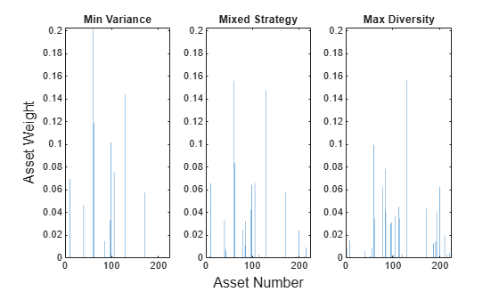
In this plot, the penalized strategy weights are between the minimum variance portfolio and the MDP. This result is the same as with the HH penalty where choosing returns the minimum variance solution and values of return asset weights that range from the minimum variance behavior to the MDP behavior.
Equal Risk Contribution (ERC) Portfolio
The diversification index associated with the equal risk contribution (ERC) portfolio is defined as
This index is related to a convex reformulation shown by Maillard [1] that is used to compute the ERC portfolio. The authors show that the ERC portfolio can be obtained by solving the following optimization problem
and defining , the ERC portfolio with default constraints, as , where can be any constant.
The purpose of the ERC portfolio is to select the assets weights in such a way that the risk contribution of each asset to the portfolio volatility is the same for all assets.
% ERC portfolio
ERCprob = optimproblem(ObjectiveSense="minimize");

% Variables
% Surrogate portfolio weights
y = optimvar("y",nX,1,LowerBound=0); % y >= 0 (long-only portfolio)

% Constraints
% Log constraint
ERCprob.Constraints.logSumIneq = sum(log(y)) >= 1;

% Objective
%   min y'*Sigma*y
ERCprob.Objective = y'*p.AssetCovar*y;

% Solve a nonlinear problem for the ERC portfolio
opts = optimoptions("fmincon",Display="none"); % No output display
w0.y = wMinVar; % Define starting point for fmincon
[wERC,fERC] = solve(ERCprob,w0,Options=opts);
xERC = wERC.y/sum(wERC.y);
The portfolio that minimizes the variance with the ERC penalty is .
Similar to the case for the MDP penalized formulation, there exists a such that the ERC problem and its penalized version are equivalent.
% ERC penalty parameter
lambdaERC = 3e-6; % lambdaERC is so small because the log of a number
                  % close to zero (the portfolio weights) is large.
% Variance + Equal Risk Contribution (ERC)
diverseProb.Objective = x'*p.AssetCovar*x - lambdaERC*sum(log(x));
% Solution that accounts for risk and ERC diversification
[wERCMix,fERCMix] = solve(diverseProb,wHH,Options=opts);
Plot the weights distribution for the minimum variance portfolio, the ERC, and the penalized strategy.
% Plot different strategies
plotAssetAllocationChanges(wMinVar,wERCMix.x,xERC)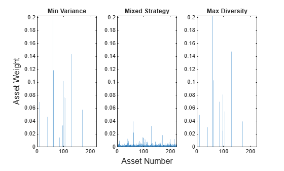
Comparable to the two diversification measures above, here the penalized strategy weights are between the minimum variance portfolio and the ERC portfolio. Choosing returns the minimum variance solution and the values of return asset weights that range from the minimum variance behavior to the ERC portfolio behavior.
Compare Diversification Strategies
Compute the number of assets that are selected in each portfolio. Assume that an asset is selected if the weight associated to that asset is above a certain threshold.
% Build a weights table
varNames = ["MinVariance","MixedHH","HH","MixedMDP","MDP", ...
    "MixedERC","ERC"];
weightsTable = table(wMinVar,wHHMix.x,wHH.x,wMDPMix.x,xMDP, ...
    wERCMix.x,xERC,VariableNames=varNames);
% Number of assets with nonzero weights
cutOff = 1e-3; % Weights below cut-off point are considered zero.
[reweightedTable,TnonZero] = tableWithNonZeroWeights(weightsTable, ...
    cutOff,varNames);
display(TnonZero)
TnonZero=1×7 table
                       MinVariance    MixedHH    HH     MixedMDP    MDP    MixedERC    ERC
                       ___________    _______    ___    ________    ___    ________    ___

    Nonzero weights        11           104      225       23       28       225       12
As discussed above, the HH penalty goal is to obtain more evenly weighted portfolios. The portfolio that maximizes the HH diversity (and corresponds to the EW portfolio when only the default constraints are selected) has the largest number of assets selected and the weights of these assets are closer together. This latter quality is observed in the following boxchart. Also, the strategy that adds the HH index as a penalty function to the objective has a larger number of assets than the minimum variance portfolio but less than the portfolio that maximizes HH diversity. The ERC portfolio also selects all the assets because all weights need to be nonzero in order to have some risk contribution.
% Boxchart of portfolio's weights
figure;
matBoxPlot = reweightedTable.Variables;
matBoxPlot(matBoxPlot == 0) = NaN;
boxchart(matBoxPlot)
xticklabels(varNames)
title("Weights Distribution")
xlabel("Strategies")
ylabel("Weight")
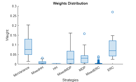
This boxchart shows the spread of the assets' positive weights for the different portfolios. As previously discussed, the weights of the portfolio that maximize the HH diversity are all the same. If the portfolio had other types of constraints, the weights would not all be the same but they would have the lowest variance. The ERC portfolio weights also have a small variance. In fact, you can observe as the number of assets increases, the variance of the ERC portfolio weights becomes smaller.
The weights variability of the MDP is smaller than the variability of the minimum variance weights. However, it is not necessarily true that the MDP's weights will have less variability than the minimum variance weights because the goal of the MDP is not to obtain equally weighted assets, but to distribute the correlation of each asset with its portfolio evenly.
% Compute and plot the risk contribution of each individual
% asset to the portfolio
riskContribution = portfolioRiskContribution(p.AssetCovar,...
    weightsTable.Variables);
% Remove small contributions
riskContribution(riskContribution < 1e-3) = NaN;

% Compare percent contribution to portfolio risk
boxchart(riskContribution)
xticklabels(varNames)
title("Percent Contributions to Portfolio Risk")
xlabel("Strategies")
ylabel("PCRs")
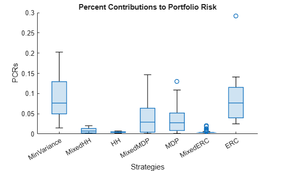
This boxchart shows the percent risk contribution of each asset to the total portfolio risk. The percent risk contribution is computed as
As expected, all the ERC portfolio assets have the same risk contribution to the portfolio. As discussed after the weights distribution plot, if the problem had other types of constraints, the risk contribution of the ERC portfolio would not be the same for all assets but they would have the lowest variance. Also, the behavior shown in this picture is similar to the behavior shown by the weights distribution.
% Compute and plot the correlation of each individual asset to its
% portfolio
corrAsset2Port = correlationInfo(p.AssetCovar,...
    weightsTable.Variables);
% Boxplot of assets to portfolio correlations
figure
boxchart(corrAsset2Port)
xticklabels(varNames)
title("Correlation of Individual Assets to Their Portfolio")
xlabel("Strategies")
ylabel("Correlation")
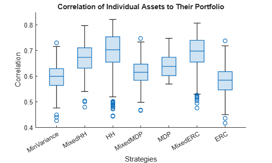
This boxchart shows the distribution of the correlations of each asset with its respective portfolio. The correlation of asset to its portfolio is computed with the following formula:
The MDP is the portfolio whose correlations are closer together and this is followed by the strategy that uses the MDP penalty term. In fact, if the portfolio problem allowed negative weights, then all the assets of the MDP would have the same correlation to its portfolio. Also, both the HH(EW) and ERC portfolios have almost the same correlation variability.
References
Maillard, S., Roncalli, T., & Teïletche, J. "The Properties of Equally Weighted Risk Contribution Portfolios." The Journal of Portfolio Management, 36(4), 2010, pp. 60-70.
Richard, J. C., & Roncalli, T. "Smart Beta: Managing Diversification of Minimum Variance Portfolios." Risk-Based and Factor Investing. Elsevier, 2015, pp. 31-63.
Tütüncü, R., Peña, J., Cornuéjols, G. Optimization Methods in Finance. United Kingdom: Cambridge University Press, 2018.
Local Functions
function [] = plotAssetAllocationChanges(wMinVar,wMix,wMaxDiv)
% Plots the weights' allocation from the strategies shown before

figure
t = tiledlayout(1,3);
nexttile
bar(wMinVar')
axis([0 225 0 0.203])
title("Min Variance")
nexttile
bar(wMix')
axis([0 225 0 0.203])
title("Mixed Strategy")
nexttile
bar(wMaxDiv')
axis([0 225 0 0.203])
title("Max Diversity")
ylabel(t,"Asset Weight")
xlabel(t,"Asset Number")

end

function [weightsTable,TnonZero] = ...
    tableWithNonZeroWeights(weightsTable,cutOff,varNames)
% Creates a table with the number of nonzero weights for each strategy

% Select only meaningful weights
funSelect = @(x) (x >= cutOff).*x./sum(x(x >= cutOff));
weightsTable = varfun(funSelect,weightsTable);

% Number of assets with positive weights
funSum = @(x) sum(x > 0);
TnonZero = varfun(funSum,weightsTable);
TnonZero.Properties.VariableNames = varNames;
TnonZero.Properties.RowNames = "Nonzero weights";

end

function [corrAsset2Port] = correlationInfo(Sigma,portWeights)
% Returns a matrix with the correlation of each individual asset to its
% portfolio

nX = size(portWeights,1); % Number of assets
nP = size(portWeights,2); % Number of portfolios

auxM = eye(nX);
corrAsset2Port = zeros(nX,nP);
for j = 1:nP
    % Portfolio's standard deviation
    sigmaPortfolio = sqrt(portWeights(:,j)'*Sigma*portWeights(:,j));
    for i = 1:nX
        % Assets's standard deviation
        sigmaAsset = sqrt(Sigma(i,i));
        % Asset to portfolio correlation
        corrAsset2Port(i,j) = (auxM(:,i)'*Sigma*portWeights(:,j))/...
            (sigmaAsset*sigmaPortfolio);
    end
end

end

function [riskContribution] = portfolioRiskContribution(Sigma,...
    portWeights)
% Returns a matrix with the risk contribution of each asset to
% the underlying portfolio.

nX = size(portWeights,1); % Number of assets
nP = size(portWeights,2); % Number of portfolios

riskContribution = zeros(nX,nP);
for i = 1:nP
    weights = portWeights(:,i);
    % Portfolio variance
    portVar = weights'*Sigma*weights;
    % Marginal constribution to portfoli risk (MCR)
    margRiskCont = weights.*(Sigma*weights)/sqrt(portVar);
    % Percent contribution to portfolio risk
    riskContribution(:,i) = margRiskCont/sqrt(portVar);
end

end
See Also
Portfolio (Financial Toolbox)
Topics
- Problem-Based Optimization Workflow
- Diversify Portfolios Using Custom Objective (Financial Toolbox)