Large System of Nonlinear Equations with Jacobian Sparsity Pattern
This example shows how to supply a Jacobian sparsity pattern to solve a large sparse system of equations effectively. The example uses the objective function, defined for a system of n equations,
The equations to solve are , . The example uses . The nlsf1a helper function at the end of this example implements the objective function .
In the example Large Sparse System of Nonlinear Equations with Jacobian, which solves the same system, the objective function has an explicit Jacobian. However, sometimes you cannot compute the Jacobian explicitly, but you can determine which elements of the Jacobian are nonzero. In this example, the Jacobian is tridiagonal, because the only variables that appear in the definition of are , , and . So the only nonzero parts of the Jacobian are on the main diagonal and its two neighboring diagonals. The Jacobian sparsity pattern is a matrix whose nonzero elements correspond to (potentially) nonzero elements in the Jacobian.
Create a sparse -by- tridiagonal matrix of ones representing the Jacobian sparsity pattern. (For an explanation of this code, see spdiags.)
n = 1000;
e = ones(n,1);
Jstr = spdiags([e e e],-1:1,n,n);
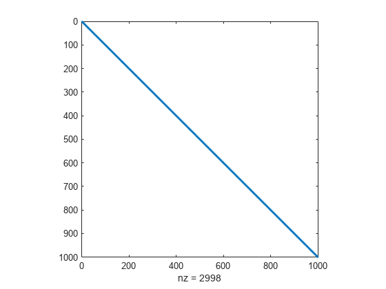
View the structure of Jstr.
spy(Jstr)
Set fsolve options to use the "trust-region" algorithm, which is the only fsolve algorithm that can use a Jacobian sparsity pattern.
options = optimoptions("fsolve",Algorithm="trust-region",JacobPattern=Jstr);
Set the initial point x0 to a vector of –1 entries.
x0 = -1*ones(n,1);
Solve the problem.
[x,fval,exitflag,output] = fsolve(@nlsf1a,x0,options);
Equation solved.

fsolve completed because the vector of function values is near zero
as measured by the value of the function tolerance, and
the problem appears regular as measured by the gradient.

<stopping criteria details>
Examine the resulting residual norm and the number of function evaluations that fsolve takes.
disp(norm(fval))
1.0522e-09
disp(output.funcCount)
25
The residual norm is near zero, indicating that fsolve solves the problem correctly. The number of function evaluations is fairly small, just around two dozen. Compare this number of function evaluations to the number without a supplied Jacobian sparsity pattern.
options = optimoptions("fsolve",Algorithm="trust-region");
[x,fval,exitflag,output] = fsolve(@nlsf1a,x0,options);
Equation solved.

fsolve completed because the vector of function values is near zero
as measured by the value of the function tolerance, and
the problem appears regular as measured by the gradient.

<stopping criteria details>
disp(norm(fval))
1.0657e-09
disp(output.funcCount)
5005
The solver reaches essentially the same solution as before, but takes thousands of function evaluations to do so.
Helper Function
This code creates the nlsf1a helper function.
function F = nlsf1a(x)
% Evaluate the vector function
n = length(x);
F = zeros(n,1);
i = 2:(n-1);
F(i) = (3-2*x(i)).*x(i)-x(i-1)-2*x(i+1) + 1;
F(n) = (3-2*x(n)).*x(n)-x(n-1) + 1;
F(1) = (3-2*x(1)).*x(1)-2*x(2) + 1;
end