Minimize Search Range in Grid-based Lidar Scan Matching Using IMU
This example shows how to use an inertial measurement unit (IMU) to minimize the search range of the rotation angle for scan matching algorithms. IMU sensor readings are used to estimate the orientation of the vehicle, and specified as the initial guess for the matchScansGrid function. This method of initial pose estimation is compared to the base algorithm with assumes an initial guess of [0 0 0].
Load Logged Data
Load the MAT file, loggedLidarAndIMUData.mat.This file contains lidar scans, accelerometer readings, and gyroscopes readings, and the corresponding timestamps.
rng(1); % Fixed RNG seed for repeatibility
load('loggedLidarAndIMUData', ...
    'tLidar', 'lidarScans', ...
    'imuFs', 'tIMU', 'accel', 'gyro');

startIdx = 1;
endIdx = numel(lidarScans)-1;
Sync IMU Time Indices with Lidar Time Indices
The IMU and lidar update at different sampling rates. Create an array that maps lidar to IMU indices.
lidarToIMUIndices = zeros(size(tLidar));
for i = 1:numel(tLidar)
    [~, lidarToIMUIndices(i)] = min(abs(tLidar(i) - tIMU));
end
Estimate Yaw from IMU
Estimate the orientation from the accelerometer and gyroscope readings as a quaternion using the imufilter object. Then, calculate the relative yaws between successive lidar scans by converting the quaternions to Euler angles.
orientFilt = imufilter('SampleRate', imuFs);
q = orientFilt(accel, gyro);

% Calculate relative yaws
eulerAngs = euler(q(lidarToIMUIndices(1+(startIdx:endIdx))) ...
    .* conj(q(lidarToIMUIndices(startIdx:endIdx))), 'ZYX', 'frame');
imuYaws = eulerAngs(:,1);
Run Scan Matching and Log Results
Run the matchScansGrid function with two different options:
Default initial guess and search range
Initial guess based on IMU sensor readings with a small search range
Iterate through all the lidar scans readings, running matchScansGrid with each pair of sequential scans. Log the processing times for each function call and the relative pose outputs from scan matching. To visualize the transformed scans based on the solution, set plotSolutions to 1. However, in this example, the difference in pose between the two different options is not noticeable.
smallSearchRange = pi/8;
plotSolutions = 0;

% Initialize time values and relative pose arrays
timeDefaultSearch = NaN(endIdx - startIdx + 1,1);
timeSmallSearchWithIMU = NaN(endIdx - startIdx + 1,1);
allRelPosesDefault = NaN(endIdx - startIdx + 1,3);
allRelPosesIMU = NaN(endIdx - startIdx + 1,3);

for idx = startIdx:endIdx
    scan1 = lidarScans(idx);
    scan2 = lidarScans(idx+1);

    yaw = imuYaws(idx);
    initGuess = [0 0 yaw];

    % Run scan matching with default values.
    tic;
    relPose = matchScansGrid(scan2, scan1);
    timeDefaultSearch(idx) = toc;

    allRelPosesDefault(idx,:) = relPose;

    % Run scan matching with IMU-based initial yaw and small search range.
    tic;
    relPose = matchScansGrid(scan2, scan1, 'InitialPose', initGuess, ...
        'RotationSearchRange', smallSearchRange);
    timeSmallSearchWithIMU(idx) = toc;
    allRelPosesIMU(idx,:) = relPose;

    % Set plot solutions to 1 to turn on scan visualization.
    if plotSolutions == 1
        figure(cfg,'Visibile','on')
        plot(scan1)
        hold on
        plot(transformScan(scan2, allRelPosesDefault(idx,:)))
        plot(transformScan(scan2, allRelPosesIMU(idx,:)))
        hold off
        legend('Ref Scan','Default', ...
            'Small Search Range + IMU',...
            'Location','northwest')
        title(sprintf('Matched Lidar Scans %d and %d', i, i+1))
    end

end
Compare Results
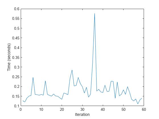
Visualize and compare the scan matching results. Show the total processing time as a bar chart. Then, compare each iteration's time.
figure
title('Scan Matching Processing Time')
bar(categorical({'Default','IMU + Small Search'}), ...
    [sum(timeDefaultSearch),sum(timeSmallSearchWithIMU)])
ylabel('time (s)')

figure
title('Difference in Interation Time')
plot(startIdx:endIdx,(timeDefaultSearch - timeSmallSearchWithIMU))
ylabel('Time (seconds)')
xlabel('Iteration')

Based on the timing results, specifying IMU sensor readings as an estimate to the scan matching algorithm improves the time of each iteration. As a final step, you can verify the difference in estimate pose is not significant. For this example, all poses from matchScansGrid are the same.
figure
title('Difference in Pose Values')
plot(allRelPosesDefault-allRelPosesIMU)
legend('X','Y','Theta')
