Improving Control Performance with Look-Ahead (Previewing)

This example shows how to design a model predictive controller with look-ahead (previewing) on reference and measured disturbance trajectories.

Define Plant Model

Define the plant model as a linear time invariant system with two inputs (one manipulated variable and one measured disturbance) and one output.

plant = ss(tf({1,1},{[1 .5 1],[1 1]}),'min');

Get the state-space matrices of the plant model, set a sampling time of 0.2 s, get the discrete-time matrices, and specify the initial condition.

[A,B,C,D] = ssdata(plant);              % continuous time ss realization
Ts = 0.2;                               % sampling time
[Ad,Bd,Cd,Dd] = ssdata(c2d(plant,Ts));  % discrete time ss realization
x0 = [0;0;0];                           % initial condition

Design Model Predictive Controller

Define type of input signals.

plant = setmpcsignals(plant,'MV',1,'MD',2);

Create the mpc object.

p = 20;                         % prediction horizon
m = 10;                         % control horizon
mpcobj = mpc(plant,Ts,p,m);
% Specify MV constraints.
mpcobj.MV = struct('Min',0,'Max',2);
% Specify weights
mpcobj.Weights = struct('MV',0,'MVRate',0.1,'Output',1);

-->"Weights.ManipulatedVariables" is empty. Assuming default 0.00000.
-->"Weights.ManipulatedVariablesRate" is empty. Assuming default 0.10000.
-->"Weights.OutputVariables" is empty. Assuming default 1.00000.

Simulate Closed Loop Using the sim Command

Tstop = 30;                     % simulation time.
time = (0:Ts:(Tstop+p*Ts))';    % time vector
r = double(time>10);            % reference signal
v = -double(time>20);           % measured disturbance signal

Use the mpcsimopt object to turn on previewing feature in the closed-loop simulation.

params = mpcsimopt(mpcobj);
params.MDLookAhead='on';
params.RefLookAhead='on';

Simulate in MATLAB® with the MPC Toolbox sim command.

YY1 = sim(mpcobj,Tstop/Ts+1,r,v,params);

-->Converting model to discrete time.
-->Assuming output disturbance added to measured output #1 is integrated white noise.
-->"Model.Noise" is empty. Assuming white noise on each measured output.

Simulate Using the mpcmove Command

Create array to store the closed-loop outputs.

YY2 = [];
% Create variables to store current states of plant and controller
x = x0;                   % initial plant state
xmpc = mpcstate(mpcobj);  % pointer to current controller state

Start simulation loop

for ct=0:round(Tstop/Ts)
    % Plant equations: output update
    y = C*x + D(:,2)*v(ct+1);
    % Store output signals
    YY2 = [YY2,y]; %#ok<*AGROW>
    % Compute MPC law. Extracts references r(t+1),r(t+2),...,r(t+p) and
    % measured disturbances v(t),v(t+1),...,v(t+p) for previewing.
    u = mpcmove(mpcobj,xmpc,y,r(ct+2:ct+p+1),v(ct+1:ct+p+1));
    % Plant equations: state update
    x = Ad*x+Bd(:,1)*u+Bd(:,2)*v(ct+1);
end

Plot results.

figure
t = 0:Ts:Tstop;
plot(t,r(1:length(t)),'c:',t,YY1,'r-',t,YY2,'bo');
xlabel('Time');
ylabel('Plant Output');
legend( ...
    {'Reference'; 'From sim command'; 'From mpcmove command'}, ...
    Location="SouthEast");
grid

The responses are identical.

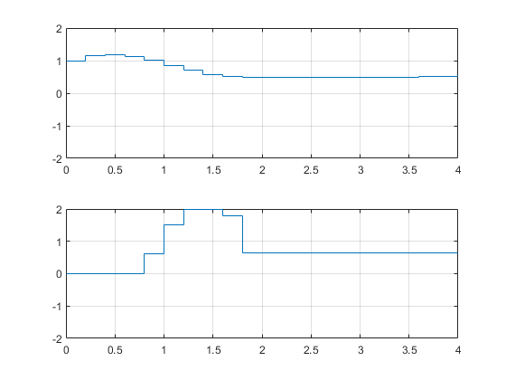
Optimal predicted trajectories are returned by mpcmove. Assume to you start from the current state and have a set-point change to 0.5 in 5 steps, and assume the measured disturbance has disappeared.

r1 = [ones(5,1);0.5*ones(p-5,1)];
v1 = zeros(p+1,1);
[~,Info] = mpcmove(mpcobj,xmpc,y,r1(1:p),v1(1:p+1));

Extract the optimal predicted trajectories and plot them.

topt = Info.Topt;
yopt = Info.Yopt;
uopt = Info.Uopt;
figure
subplot(211)
title('Optimal sequence of predicted outputs')
stairs(topt,yopt);
grid
axis([0 p*Ts -2 2]);
subplot(212)
title('Optimal sequence of manipulated variables')
stairs(topt,uopt);
axis([0 p*Ts -2 2]);
grid

Obtain LTI Representation of MPC Controller with Previewing

When the constraints are not active, the MPC controller behaves like a linear controller. You can get the state-space form of the MPC controller, with y, [r(t+1);r(t+2);...;r(t+p)], and [v(t);v(t+1);...;v(t+p)] as inputs to the controller.

Get state-space matrices of linearized controller.

LTI = ss(mpcobj,'rv','on','on');
[AL,BL,CL,DL] = ssdata(LTI);

Create array to store closed-loop outputs.

YY3 = [];
% Setup initial state of the MPC controller
x = x0;
xL = [x0;0;0];

Start main simulation loop

for ct=0:round(Tstop/Ts)

    % Plant output update
    y = Cd*x + Dd(:,2)*v(ct+1);

    % Save output and refs value
    YY3 =[YY3,y];

    % Compute the linear MPC control action
    u = CL*xL + DL*[y;r(ct+2:ct+p+1);v(ct+1:ct+p+1)];
    % Note that the optimal move provided by MPC would be:
    % mpcmove(mpcobj,xmpc,y,ref(t+2:t+p+1),v(t+1:t+p+1));

    % Plant update
    x = Ad*x + Bd(:,1)*u + Bd(:,2)*v(ct+1);

    % Controller update
    xL = AL*xL + BL*[y;r(ct+2:ct+p+1);v(ct+1:ct+p+1)];
end

Plot results.

figure
plot(t,r(1:length(t)),'c:',t,YY3,'r-');
xlabel('Time');
ylabel('Plant Output');
legend({'Reference';'Unconstrained MPC'},'Location','SouthEast');
grid

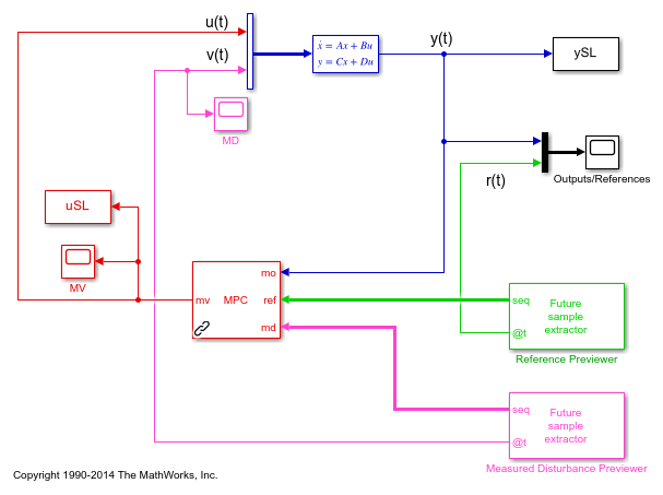
Simulate Using Simulink®

To run this example, Simulink® is required.

if ~mpcchecktoolboxinstalled('simulink')
    disp('Simulink(R) is required to run this example.')
    return
end

time = (0:Ts:(Tstop+p*Ts))'; % time vector
r = double(time>10); % reference signal
v = -double(time>20); % measured disturbance signal

% Define the reference signal in structure
ref.time = time;
ref.signals.values = r;

% Define the measured disturbance
md.time = time;
md.signals.values = v;

% Open Simulink model
mdl = 'mpc_preview';
open_system(mdl)

% Simulate the model using the Simulink |sim| command
sim(mdl,Tstop);

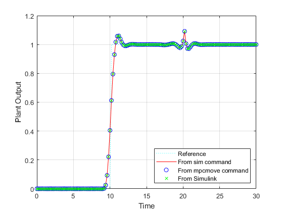
Plot results.

figure
t = 0:Ts:Tstop;
plot(t,r(1:length(t)),'c:',t,YY1,'r-',t,YY2,'bo',t,ySL,'gx');
xlabel('Time');
ylabel('Plant Output');
legend({'Reference'; ...
    'From sim command'; ...
    'From mpcmove command'; ...
    'From Simulink'}, ...
    Location="SouthEast");
grid

The responses are identical.