buildMEX

Build MEX file that solves an MPC control problem

Syntax

mexLinFcn = buildMEX(mpcobj,mexName,coreData,stateData,onlineData)

mexNlnFcn = buildMEX(nlobj,mexName,coreData,onlineData)

mexFcn = buildMEX(nlobj,mexName,coreData,onlineData,mexConfig)

Description

Linear MPC

mexLinFcn = buildMEX(mpcobj,mexName,coreData,stateData,onlineData) builds a MEX file that solves a linear MPC control problem faster than mpcmove. The MEX file is created in the current working folder.

Nonlinear MPC

mexNlnFcn = buildMEX(nlobj,mexName,coreData,onlineData) builds a MEX file that solves a nonlinear MPC control problem faster than nlmpcmove. The MEX file is created in the current working folder.

mexFcn = buildMEX(nlobj,mexName,coreData,onlineData,mexConfig) generates a MEX function using the code generation configuration object mexConfig. Use this syntax to customize your MEX code generation.

Examples

Simulate Linear MPC Controller Using MEX File

Create a plant model and design an MPC controller for the plant, with sample time 0.1.

plant = drss(1,1,1);plant.D = 0;
mpcobj = mpc(plant,0.1);

-->"PredictionHorizon" is empty. Assuming default 10.
-->"ControlHorizon" is empty. Assuming default 2.
-->"Weights.ManipulatedVariables" is empty. Assuming default 0.00000.
-->"Weights.ManipulatedVariablesRate" is empty. Assuming default 0.10000.
-->"Weights.OutputVariables" is empty. Assuming default 1.00000.

Simulate the plant using mpcmove for 5 steps.

x = 0;
xc = mpcstate(mpcobj);

-->No sample time in plant model. Assuming controller's sample time of 0.1.
-->Assuming output disturbance added to measured output #1 is integrated white noise.
-->"Model.Noise" is empty. Assuming white noise on each measured output.

for i=1:5
    % Update plant output.
    y = plant.C*x;
    % Compute control actions.
    u = mpcmove(mpcobj,xc,y,1);
    % Update plant state.
    x = plant.A*x + plant.B*u;
end

Display the final value of the plant output, input and next state.

[y u x]

ans = 1×3

    0.9999    0.3057   -2.3063

Generate data structures and build mex file.

[coreData,stateData,onlineData] = getCodeGenerationData(mpcobj);
mexfun = buildMEX(mpcobj, 'myMPCMex', coreData, stateData, onlineData);

Generating MEX function "myMPCMex" from linear MPC to speed up simulation.
Code generation successful.

MEX function "myMPCMex" successfully generated.

Simulate the plant using the mex file myMPCmex, which you just generated, for 5 steps.

x=0;
for i = 1:5
    % Update plant output.
    y = plant.C*x;
    % Update measured output in online data.
    onlineData.signals.ym = y;
    % Update reference signal in online data.
    onlineData.signals.ref = 1;
    % Compute control actions.
    [u,stateData] = myMPCMex(stateData,onlineData);
    % Update plant state.
    x = plant.A*x + plant.B*u;
end

Display the final value of the plant output, input and next state.

[y u x]

ans = 1×3

    0.9999    0.3057   -2.3063

Simulate Nonlinear MPC Controller Using MEX File

Create a nonlinear MPC controller with four states, two outputs, and one input.

nlobj = nlmpc(4,2,1);

Zero weights are applied to one or more OVs because there are fewer MVs than OVs.

Specify the sample time and horizons of the controller.

Ts = 0.1;
nlobj.Ts = Ts;
nlobj.PredictionHorizon = 10;
nlobj.ControlHorizon = 5;

Specify the state function for the controller, which is in the file pendulumDT0.m. This discrete-time model integrates the continuous-time model defined in pendulumCT0.m using a multistep forward Euler method.

nlobj.Model.StateFcn = "pendulumDT0";
nlobj.Model.IsContinuousTime = false;

The prediction model uses an optional parameter Ts to represent the sample time. Specify the number of parameters and create a parameter vector.

nlobj.Model.NumberOfParameters = 1;
params = {Ts};

Specify the output function of the model, passing the sample time parameter as an input argument.

nlobj.Model.OutputFcn = "pendulumOutputFcn";

Define standard constraints for the controller.

nlobj.Weights.OutputVariables = [3 3];
nlobj.Weights.ManipulatedVariablesRate = 0.1;
nlobj.OV(1).Min = -10;
nlobj.OV(1).Max = 10;
nlobj.MV.Min = -100;
nlobj.MV.Max = 100;

Validate the prediction model functions.

x0 = [0.1;0.2;-pi/2;0.3];
u0 = 0.4;
validateFcns(nlobj,x0,u0,[],params);

Model.StateFcn is OK.
Model.OutputFcn is OK.
Analysis of user-provided model, cost, and constraint functions complete.

Only two of the plant states are measurable. Therefore, create an extended Kalman filter for estimating the four plant states. Its state transition function is defined in pendulumStateFcn.m and its measurement function is defined in pendulumMeasurementFcn.m.

EKF = extendedKalmanFilter(@pendulumStateFcn,@pendulumMeasurementFcn);

Define initial conditions for the simulation, initialize the extended Kalman filter state, and specify a zero initial manipulated variable value.

x0 = [0;0;-pi;0];
y0 = [x0(1);x0(3)];
EKF.State = x0;
mv0 = 0;

Create code generation data structures for the controller, specifying the initial conditions and parameters.

[coreData,onlineData] = getCodeGenerationData(nlobj,x0,mv0,params);

Specify the output reference value in the online data structure.

onlineData.ref = [0 0];

Build a MEX function for solving the nonlinear MPC control problem. The MEX function is created in the current working directory.

mexFcn = buildMEX(nlobj,"myController",coreData,onlineData);

Generating MEX function "myController" from nonlinear MPC to speed up simulation.
Code generation successful.

MEX function "myController" successfully generated.

Run the simulation for 10 seconds. During each control interval:

1. Correct the previous prediction using the current measurement.

2. Compute optimal control moves using the MEX function. This function returns the computed optimal sequences in onlineData. Passing the updated data structure to the MEX function in the next control interval provides initial guesses for the optimal sequences.

3. Predict the model states.

4. Apply the first computed optimal control move to the plant, updating the plant states.

5. Generate sensor data with white noise.

6. Save the plant states.

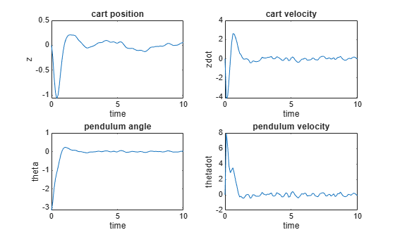
mv = mv0;
y = y0;
x = x0;
Duration = 10;
xHistory = x0;
for ct = 1:(Duration/Ts)
    % Correct previous prediction
    xk = correct(EKF,y);
    % Compute optimal control move
    [mv,onlineData] = myController(xk,mv,onlineData);
    % Predict prediction model states for the next iteration
    predict(EKF,[mv; Ts]);
    % Implement first optimal control move
    x = pendulumDT0(x,mv,Ts);
    % Generate sensor data
    y = x([1 3]) + randn(2,1)*0.01;
    % Save plant states
    xHistory = [xHistory x];
end

Plot the resulting state trajectories.

figure
subplot(2,2,1)
plot(0:Ts:Duration,xHistory(1,:))
xlabel('time')
ylabel('z')
title('cart position')
subplot(2,2,2)
plot(0:Ts:Duration,xHistory(2,:))
xlabel('time')
ylabel('zdot')
title('cart velocity')
subplot(2,2,3)
plot(0:Ts:Duration,xHistory(3,:))
xlabel('time')
ylabel('theta')
title('pendulum angle')
subplot(2,2,4)
plot(0:Ts:Duration,xHistory(4,:))
xlabel('time')
ylabel('thetadot')
title('pendulum velocity')

Input Arguments

mpcobj — Model predictive controller

mpc object | explicitMPC object

Model predictive controller, specified as one of the following:

• mpc object — Implicit MPC controller

• explicitMPC object — Explicit MPC controller created using generateExplicitMPC.

nlobj — Nonlinear model predictive controller

nlmpc object | nlmpcMultistage object

Nonlinear model predictive controller, specified as an nlmpc or nlmpcMultistage object.

Your controller must use the default fmincon solver with the SQP algorithm. Also, your controller must not use anonymous functions for its prediction model, custom cost function, or custom constraint functions.

mexName — MEX function name

string | character vector

MEX function name, specified as a string or character vector.

coreData — Controller configuration parameters

structure

Nonlinear MPC configuration parameters that are constant at run time, specified as a structure generated using getCodeGenerationData.

stateData — Linear controller state data structure

structure

Linear controller state data structure at run time, specified as a structure generated using getCodeGenerationData.

onlineData — Initial online controller data

structure

Initial online controller data, specified as a structure generated using getCodeGenerationData. For more information on setting the fields of onlineData, see nlmpcmoveCodeGeneration.

mexConfig — Code generation configuration object

MexCodeConfig object

Code generation configuration object, specified as a MexCodeConfig object.

To create the configuration object, use the following code.

mexConfig = coder.config('mex');

To customize your MEX code generation, modify the settings of this object. For example, to detect run-time memory access violations during debugging, set IntegrityChecks to true.

mexConfig.IntegrityChecks = true;

By default, to improve the performance of the generated code, checks such as IntegrityChecks and ResponsivenessChecks are disabled by buildMEX.

buildMEX overwrites the following configuration settings with the values indicated.

Configuration Setting	Value
cfg.DynamicMemoryAllocation	'AllVariableSizeArrays'
cfg.ConstantInputs	'Remove'

Output Arguments

mexLinFcn — Generated MEX function for linear MPC

function handle

Generated MEX function for linear MPC, returned as a function handle. This MEX function has the following signature.

[mv,newStateData,info] = mexLinFcn(stateData,onlineData)

The MEX function has the following input arguments, which are the same as the corresponding input arguments of mpcmoveCodeGeneration, except configData, which is embedded in mexLinFcn.

Input Argument	Description
stateData	Current state data. Structure containing the state of the linear MPC controller. For more information on setting the fields of onlineData, see mpcmoveCodeGeneration.
onlineData	Online controller data that you must update at run time, specified as a structure. Generate the initial structure using getCodeGenerationData. For more information on setting the fields of onlineData, see mpcmoveCodeGeneration.

The MEX function has the following output arguments, which are the same as the output arguments of mpcmoveCodeGeneration.

Output Argument	Description
mv	Optimal manipulated variable control action, returned as a column vector of length Nmv, where Nmv is the number of manipulated variables.
newStateData	Updated state data. Structure containing the updated state of the linear MPC controller. For more information on setting the fields of onlineData, see mpcmoveCodeGeneration.
info	Solution details, returned as a structure.

To simulate a controller using the generated MEX function, use the initial online data structure onlineData for the first control interval. For subsequent control intervals, modify the online data in newOnlineData and pass the updated structure to the MEX function as onlineData.

mexNlnFcn — Generated MEX function for nonlinear MPC

function handle

Generated MEX function for nonlinear MPC, returned as a function handle. This MEX function has the following signature.

[mv,newOnlineData,info] = mexNlnFcn(x,lastMV,onlineData)

The MEX function has the following input arguments, which are the same as the corresponding input arguments of nlmpcmoveCodeGeneration.

Input Argument	Description
x	Current prediction model states, specified as a vector of length Nx, where Nx is the number of prediction model states.
lastMV	Control signals used in plant at previous control interval, specified as a vector of length Nmv, where Nmv is the number of manipulated variables.
onlineData	Online controller data that you must update at run time, specified as a structure. Generate the initial structure using getCodeGenerationData. For more information on setting the fields of onlineData, see nlmpcmoveCodeGeneration.

The MEX function has the following output arguments, which are the same as the output arguments of nlmpcmoveCodeGeneration.

Output Argument	Description
mv	Optimal manipulated variable control action, returned as a column vector of length Nmv, where Nmv is the number of manipulated variables.
newOnlineData	Updated online controller data, returned as a structure. This structure is the same as onlineData, except that the decision variable initial guesses are updated.
info	Solution details, returned as a structure.

To simulate a controller using the generated MEX function, use the initial online data structure onlineData for the first control interval. For subsequent control intervals, modify the online data in newOnlineData and pass the updated structure to the MEX function as onlineData.

Version History

Introduced in R2020a