PMSM Constraint Curves and Their Application

Open Live Script

This example uses Motor Control Blockset™ to explain the fundamentals of constraint curves, utilization of these curves to determine operating currents, and usage of the grid of these currents in simulation or deployment environments.

The section Fundamentals of Constraint Curves of PMSM explains about the constraint curves of a Permanent Magnet Synchronous Machine (PMSM). The five curves (current limit circle, constant torque curve, MTPA curve, voltage limit curve, and MTPV curve) represent the constraints and characteristics of a motor system.

The section Using Constraint Curves explains about the applications of the constraint curves in identifying the optimal operating points to determine reference currents across d- and q-axes for a given operating speed and reference torque. This section shows you how to create lookup tables (LUTs) of the reference currents. The example explains about a group of five operating points across different regions.

The section Identifying Possible (MTPA-Field Weakening-MTPV) Control Currents shows you how to use the LUT based PMSM Control Reference block to determine the operating points in a simulation environment.

Required MathWorks Products

Motor Control Blockset
Simulink®

Fundamentals of Constraint Curves of PMSM

Constraint curves represent the operational constraints of PMSM control. Each curve corresponds to either a constraint or a characteristic behavior.

Use the following code to re-create figure 1.

pmsm=mcb_SetPMSMMotorParameters('Teknic2310P');
pmsm.Rs=0.01;
pmsm.Lq=pmsm.Ld*2;
inverter=mcb_SetInverterParameters('BoostXL-DRV8305');
mcbPMSMCharacteristics(pmsm,inverter,speed=5500,torque=0.1394);

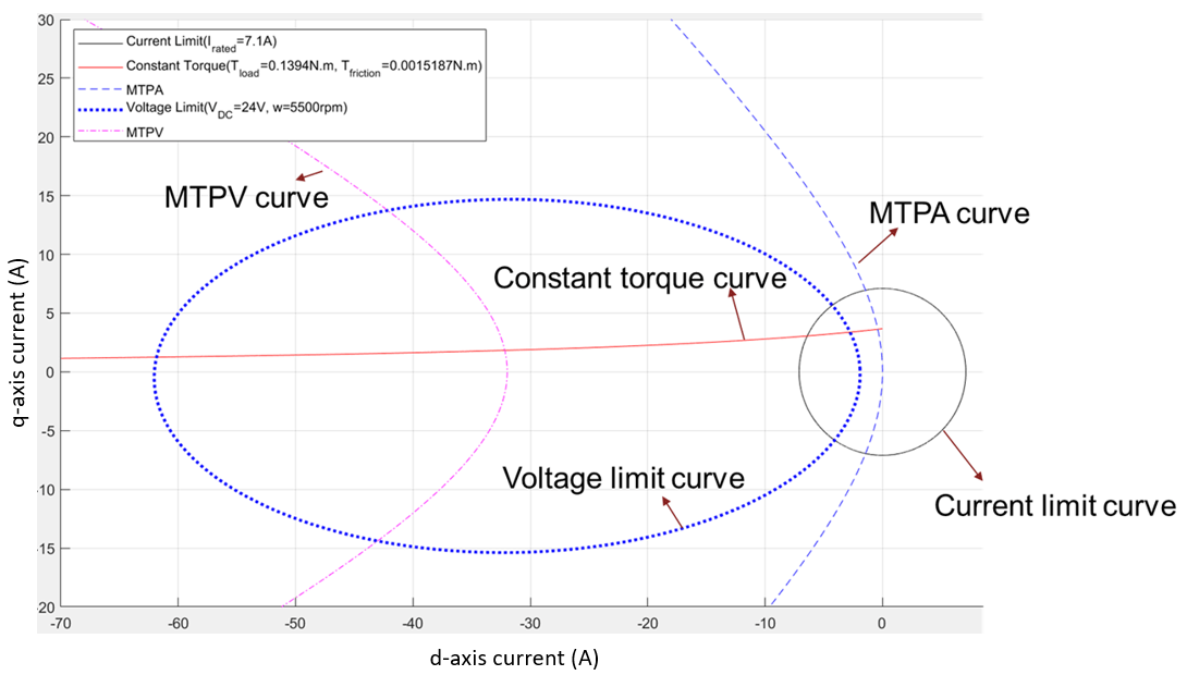
Figure 1: Representation of constraint curves of a PMSM

The d-q Frame of Reference

The d-q frame of reference is a rotating frame of reference that rotates along with the rotor. Unlike the stationary frame of reference, the d-q frame of reference simplifies the representation of the electrical quantities of a motor, such as voltages and currents.

You can measure the motor phase currents ia, ib, and ic and transform them into d-q reference frame currents (id, iq) using the rotor position. For a balanced three phase system, you can assume that the zero-sequence current is equal to zero. For more details about the Clarke and Park transformations, see Clarke and Park Transforms - MATLAB & Simulink (mathworks.com).

The d-q Current Space

This is the imaginary frame of reference with the d-axis current represented on the x-axis and the q-axis current represented on the y-axis.

You can plot the limits and characteristics of a given PMSM (when represented in terms of id and iq) in the d-q current space.

Current Limit Circle

The current limit circle is the operating limit of the system on the current. Because the net current of the system is limited and the id and iq components are orthogonal, these currents follow this relationship:

$i_{d}^{2} + i_{q}^{2} = i_{s}^{2} \leq i_{s_\max}^{2}$

where,

$i_{d}$ is the d-axis current (in amperes).
$i_{q}$ is the q-axis current (in amperes).
$i_{s}$ is the source current (in amperes).
$i_{s_\max}$ is the maximum source current (in Amperes).

Because $i_{s_\max}$ is constant for a given current constraint, the locus of all the points that satisfy this relation represents a circle.

Any point inside this circle (id, iq) has a magnitude that is less than the current limit $i_{s_\max}$ . Therefore, all the points inside the circle are valid points when considering the current constraint.

Irrespective of the motor topology (either a surface PMSM (SPMSM) or an interior PMSM (IPMSM)), the current limit circle remains a circle.

The following figure shows the plot of a current limit circle with an $i_{s_\max}$ of 7.1A.

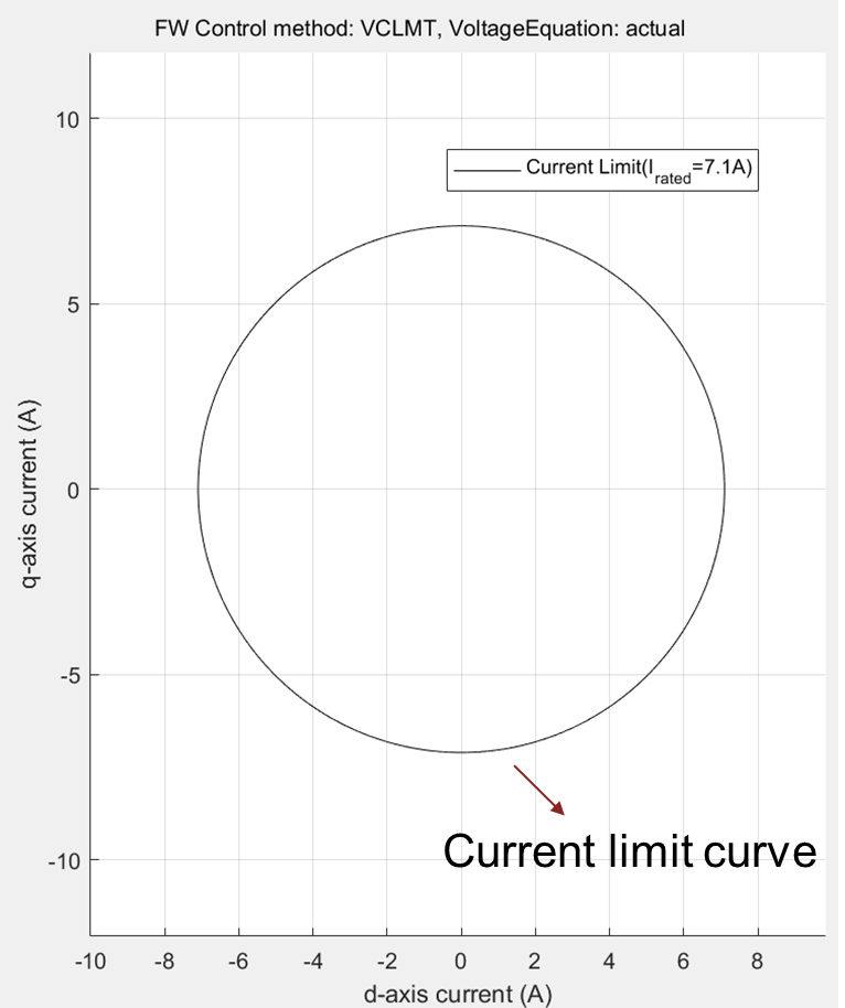
Figure 2: Current limit circle or current limit curve of a PMSM

Constant Torque Curve

Constant torque curve is a locus of all (id,iq) points that deliver an identical torque.

The torque of a PMSM includes the reluctance torque and PM torque. The following equation represents the generated torque:

$T = 1.5 p (i_{q} λ_{p m} + (L_{d} - L_{q}) i_{d} i_{q})$

where,

$p$ is the number of pole pairs in the PMSM.
$λ_{p m}$ is the permanent magnet flux linkage (weber).
$i_{d}$ and $i_{q}$ are the d-axis and q-axis currents, respectively (in amperes).
$L_{d}$ and $L_{q}$ are the d-axis and q-axis inductances, respectively (in henries).

For a given fixed torque, this equation transforms to $i_{q} = \frac{K_{1}}{K_{2} + i_{d}}$ , which represents a hyperbola.

Any (id, iq) value pair on the constant torque curve represents the currents that satisfy the load torque. To ensure that an (id,iq) value pair also satisfies constraints, you can check if this point satisfies the current constraint (inside the closed circle formed by the current limit curve).

Figure 3: Current limit circle and constant torque curve of a PMSM.

Figure 4: Current limit circle and a group of constant torque curves drawn at different torque values in an increasing order. The lighter shade of the constant torque curve represents an increasing torque.

MTPA Curve

MTPA stands for maximum torque per ampere. An MTPA curve is the locus of all points that satisfy the optimization condition providing a maximum torque for a given operating current.

You can obtain the expression for MTPA curve (using linear motor parameters) with an assumption that the partial derivative of the torque with respect to current (either id or iq) is equal to zero.

For an IPMSM, the following expression represents an MTPA trajectory:

$i_{d}^{2} + \frac{i_{d} λ_{p m}}{L_{d} - L_{q}} = i_{q}^{2}$

where,

$λ_{p m}$ is the permanent magnet flux linkage (weber).
$i_{d}$ and $i_{q}$ are the d-axis and q-axis currents respectively (in amperes).
$L_{d}$ and $L_{q}$ are the d-axis and q-axis inductances respectively (in henries).

This equation represents a parabola. All the points on the MTPA curve satisfy the condition that they provide maximum torque per operating current.

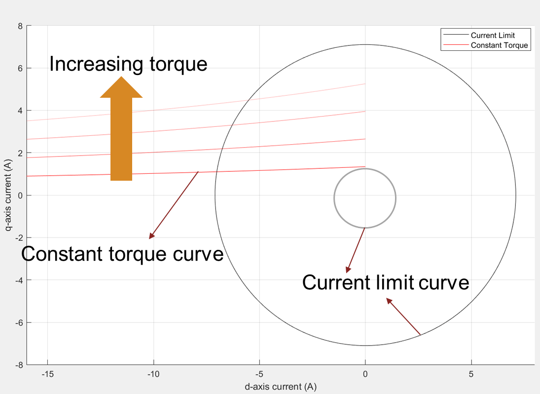
Figure 5: Current limit circle, a group of constant torque curves, and a smaller current limit circle representing the current limit for one of the constant torque curves.

When you consider the operating current as the virtual current limit for a hypothetical system and draw the constraint curves including a constant torque curve and a current limit circle, they both intersect tangentially at a single point. This point represents the maximum possible torque that you can achieve using the virtual current limit for the hypothetical system.

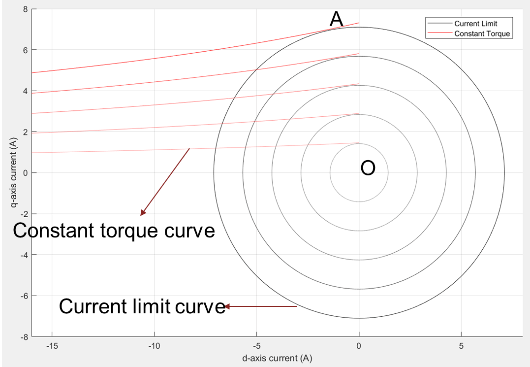
Figure 6: A group of pairs of current limit circles with different limit values and the corresponding maximum torques.

Figure 7: A group of pairs of current limit circles with different limit values with the corresponding maximum torques and the MTPA curve.

As shown in figure 7, the MTPA curve is a collection of all points that are intersecting points of current limit circles and the corresponding constant torque curves (drawn at maximum possible torque for the given current). This curve visually represents a way to understand MTPA in terms of points representing the maximum torque for a given current.

Voltage Limit Curve

Voltage limit curve is the locus of all (id,iq) points for a specified speed and voltage, due to which the system voltage, $\sqrt{v_{d}^{2} + v_{q}^{2}}$ , reaches the voltage limit, vmax.

These equations represent the phase voltages in the d-q reference frame:

$v_{d} = i_{d} R_{s} - ω_{e} λ_{Q}$ , where $λ_{Q} = L_{q} i_{q}$

$v_{q} = i_{q} R_{s} + ω_{e} λ_{D}$ , where $λ_{D} = L_{d} i_{d} + λ_{p m}$

$ω_{e} = p ω$ , where $ω = \frac{2 π N}{60}$

where,

$λ_{D}$ and $λ_{Q}$ are the d-axis and q-axis flux linkages respectively (in weber).
$λ_{p m}$ is the permanent magnet flux linkage (weber).
$i_{d}$ and $i_{q}$ are the d-axis and q-axis currents respectively (in amperes).
$v_{d}$ and $v_{q}$ are the d-axis and q-axis voltages respectively (in volts).
$L_{d}$ and $L_{q}$ are the d-axis and q-axis inductances respectively (in henries).
$p$ is the number of motor pole pairs.
$ω$ is the rotor mechanical rotational speed (in radians/ sec).
$N$ is the rotor mechanical speed (in rpm).
$ω_{e}$ is the rotor electrical rotational speed (in radians/ sec).
$R_{s}$ is the stator phase winding resistance (in ohms).

The system voltage is constrained by the operating power supply voltage and the PWM scheme. For SVPWM, the available voltage is $v_{\max} = \frac{V_{d c}}{\sqrt{3}}$ , while for Sine PWM, the available voltage is $v_{\max} = \frac{V_{d c}}{2}$ .

$v_{d}^{2} + v_{q}^{2} = v_{s}^{2} \leq v_{\max}^{2}$

where,

$v_{d}$ and $v_{q}$ are the d-axis and q-axis voltages respectively (in volts).
$v_{s}$ is the source voltage (in volts).
$v_{\max}$ is the maximum fundamental line to neutral voltage (peak) supplied to the motor (in volts).

To satisfy the voltage constraint, the system voltage, $v_{s}$ , should be equal to or less than vmax.

After replacing the vd and vq representations in the preceding equation, you get:

${(i_{d} R_{s} - ω_{e} L_{q} i_{q})}^{2} + {(i_{q} R_{s} + ω_{e} L_{d} i_{d} + ω_{e} λ_{p m})}^{2} = v_{s}^{2} \leq v_{\max^{2}}$

where,

$λ_{p m}$ is the permanent magnet flux linkage (weber).
$i_{d}$ and $i_{q}$ are the d-axis and q-axis currents respectively (in amperes).
$v_{d}$ and $v_{q}$ are the d-axis and q-axis voltages respectively (in volts).
$v_{s}$ is the source voltage (in volts).
$v_{\max}$ is the maximum fundamental line to neutral voltage (peak) supplied to the motor (in volts).
$L_{d}$ and $L_{q}$ are the d-axis and q-axis inductances respectively (in henries).
$ω_{e}$ is the rotor electrical rotational speed (in radians/ sec).
$R_{s}$ is the stator phase winding resistance (in ohms).

This equation represents a generalized ellipse.

SPMSM has Ld = Lq, while for an IPMSM, Lq > Ld, where Ld and Lq are the inductances along the d- and q-axes, respectively.

Due to the above parameter variation, the voltage limit curve of the SPMSM forms a circle, with the center away from the origin. The shift from the origin (id=0, iq=0) depends on the FluxPM, speed, Rs, Ld, and Lq motor system parameters.

Because for an IPMSM, Ld and Lq are not identical, the generated voltage limit curve is an ellipse.

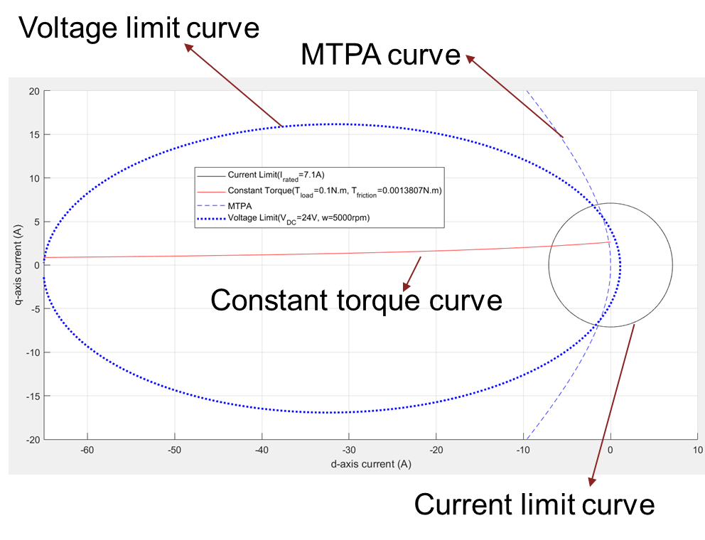
Figure 8: Current limit circle, voltage limit curve, and MTPA curve of a PMSM.

Figure 8 includes the voltage limit ellipse for a given motor. You can see that the current limit circle is centered around the origin and the voltage limit ellipse is not centered around the origin. The region of overlap between the voltage limit ellipse and the current limit circle represent the possible (id, iq) current values that satisfy both the voltage and current constraints.

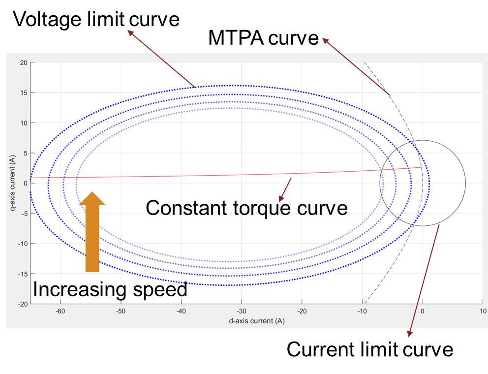
Figure 9: Current limit circle, MTPA curve, and a group of voltage limit curves drawn at different speeds. The lighter dotted blue lines represent the increasing direction of speed.

Voltage Limit Curve - Approximate Equations vs Actual Equations

A simpler form of the voltage limit curve is known as an approximate representation. In this representation, you can ignore the $i r$ component in the vd and vq equations and compensate them in the vmax term.

The following equations use approximate representation to show the phase voltages in the d-q reference frame:

$v_{d} = - ω_{e} λ_{Q}$ , where $λ_{Q} = L_{q} i_{q}$

$v_{q} = ω_{e} λ_{D}$ , where $λ_{D} = L_{d} i_{d} + λ_{p m}$

The system voltage is constrained by the operating power supply voltage and the PWM scheme. For SVPWM, the available voltage is $v_{\max} = \frac{V_{d c}}{\sqrt{3}} - i_{\max} R_{s}$ , while for Sine PWM, the available voltage is $v_{\max} = \frac{V_{d c}}{2} - i_{\max} R_{s}$ .

$v_{d}^{2} + v_{q}^{2} = v_{s}^{2} \leq v_{\max}^{2}$

The system voltage vs that is equal to or less than vmax, satisfies the voltage constraint.

After inserting vd and vq representations in the preceding equation, you get:

${(- ω_{e} L_{q} i_{q})}^{2} + {(ω_{e} L_{d} i_{d} + ω_{e} λ_{p m})}^{2} = v_{s}^{2} \leq v_{\max^{2}}$

where,

$λ_{D}$ and $λ_{Q}$ are the d-axis and q-axis flux linkages, respectively (in weber).
$λ_{p m}$ is the permanent magnet flux linkage (weber).
$i_{d}$ and $i_{q}$ are the d-axis and q-axis currents, respectively (in amperes).
$i_{\max}$ is the maximum phase current (peak) of the motor (in amperes).
$v_{d}$ and $v_{q}$ are the d-axis and q-axis voltages, respectively (in volts).
$v_{s}$ is the source voltage (in volts).
$v_{\max}$ is the maximum fundamental line to neutral voltage (peak) supplied to the motor (in volts).
$V_{d c}$ is the DC voltage supplied to the inverter (in volts).
$L_{d}$ and $L_{q}$ are the d-axis and q-axis inductances, respectively (in henries).
$ω_{e}$ is the rotor electrical rotational speed (in radians/ sec).
$R_{s}$ is the stator phase winding resistance (in ohms).

This equation represents an ellipse for an IPMSM, centered on the x-axis of the id-iq plane.

In figure 10(b), the voltage limit curve with actual equations is a tilted ellipse, while the voltage limit curve with approximate equations is an ellipse along the x-axis and centered on x-axis.

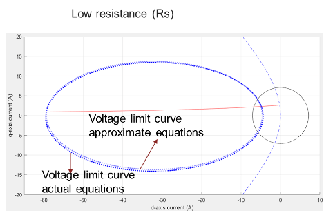
Figure 10(a): A comparison of voltage limit curves for actual and approximate equations for a system with low Rs.

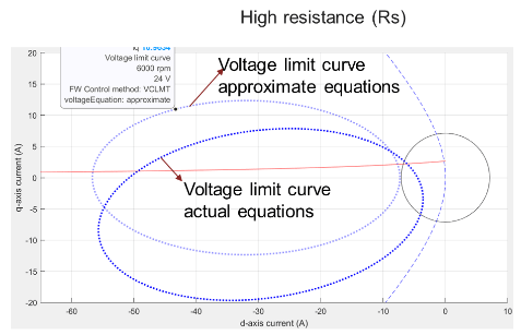
Figure 10(b): A comparison of voltage limit curves for actual and approximate equations for a system with high Rs.

MTPV Curve

MTPV stands for Maximum Torque Per Voltage. MTPV curve is a group of all points that satisfy the voltage constraint while providing the maximum possible torque. When considering the linear motor parameters, you can derive an empirical expression for the MTPV curve. However, this can become complicated when you represent the voltages in their actual form. You can derive the empirical form by equating the partial derivative of torque (with respect to the voltage (vd or vq)) to zero.

The following expression defines the MTPV curve:

$v_{d}^{2} + v_{d} K_{1} + v_{d} v_{q} K_{2} = v_{q}^{2} + v_{q} K_{3}$ , where K1, K2, and K3 are the terms involving Ld, Lq, speed, Rs, and FluxPM. This equation requires expansion into id and iq terms. However, for an SPMSM, the MTPV curve equation is $i_{d} = \frac{- (ω_{e}^{2} L λ_{p m})}{(R_{s}^{2} + ω_{e}^{2} L^{2})}$ , which is a straight line parallel to the y-axis with a position that changes based on the motor parameters and the operating speed.

where,

$λ_{p m}$ is the permanent magnet flux linkage (weber).
$i_{d}$ is the d-axis current (in amperes).
$v_{d}$ and $v_{q}$ are the d-axis and q-axis voltages, respectively (in volts).
$L_{d}$ and $L_{q}$ are the d-axis and q-axis inductances, respectively (in henries).
$L$ is the total motor inductance (in henries).
$ω_{e}$ is the rotor electrical rotational speed (in radians/ sec).
$R_{s}$ is the stator phase winding resistance (in ohms).

Figure 11: Current limit circle, MTPA curve, a group of pairs of voltage limit curves, and constant torque curves that tangentially touch the corresponding voltage limit curve.

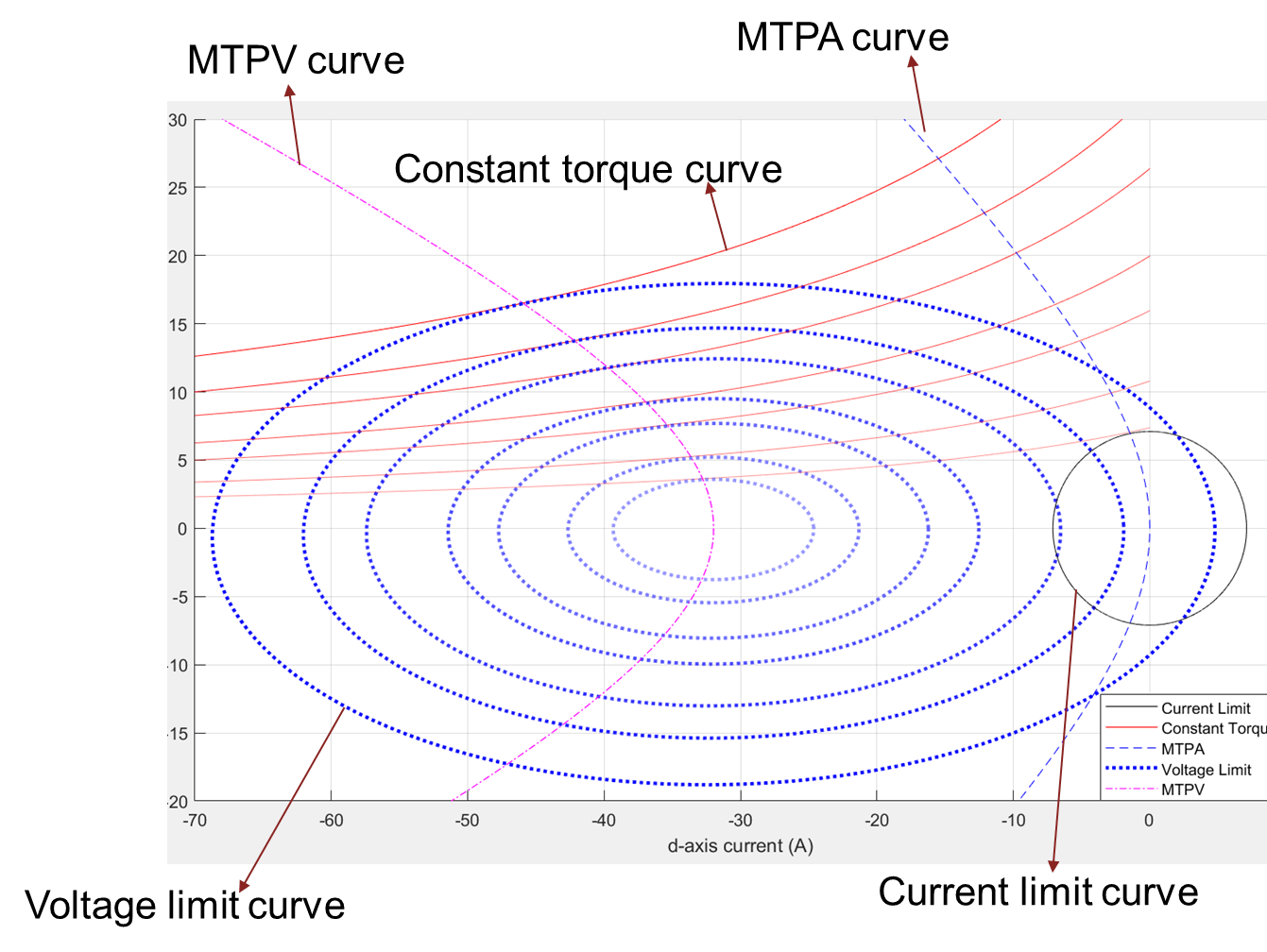
Figure 12: Current limit circle, MTPA curve, a group of pairs of voltage limit curves, constant torque curves that tangentially touch the corresponding voltage limit curve, and the MTPV curve.

Using Constraint Curves

You can use the constraint curves in multiple ways. This section lists some of these methods.

Find Maximum Operable Speed

You can find the maximum operable speed of a PMSM (either SPMSM or IPMSM) in different ways. You can either use the analytical equations or the constraint curves to find the maximum speed. Note that you can use a machine with a limited speed due to several constraints (such as efficiency, mechanical stability, and maximum required speed).

From the constraint curves, you can obtain the maximum operable speed of a machine, which is a point where the internal frictional torque (with no load torque) can be supported by the torque produced by the motor. When the speed increases beyond the maximum speed, the frictional load torque increases and the motor fails to support the load torque.

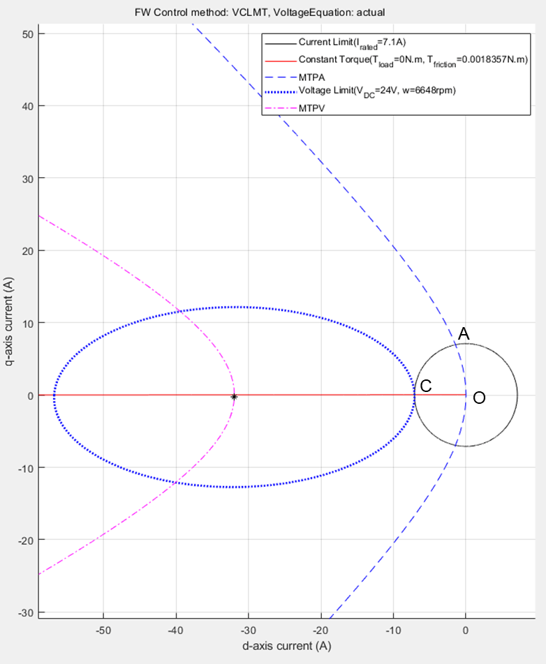
Figure 13 : Constraint curves of a PMSM, drawn at maximum operable speed, at 0 N.m. load torque.

Figure 14: Zoomed-in portion from figure 13 to show the intersection of three curves - current limit circle, voltage limit ellipse, and constant torque curve.

Figure 15: Drive characteristics of the motor that is marked with the operating points at the maximum speed.

The following code can be used to find the maximum speed of the motor.

pmsm=mcb_SetPMSMMotorParameters('Teknic2310P');
pmsm.Rs=0.01;
pmsm.Lq=pmsm.Ld*2;
inverter=mcb_SetInverterParameters('BoostXL-DRV8305');
max_speed=mcbPMSMMaxSpeed(pmsm,inverter);
disp('maximum speed is ' + string(max_speed) + ' rpm');

maximum speed is 6648 rpm

Finding Corner Speed of Motor

The rated speed of a motor is the speed at which the motor can be loaded with the rated torque, while operating at the rated voltage. This speed is also known as the corner speed because at this speed, speed-torque characteristics of a PMSM has a change of shape. For example, in figure 18, the point A marks the corner speed of the motor. This speed is also known as the base speed. You can either use the analytical equations or the constraint curves to find the corner speed.

From the constraint curves, you can determine the corner speed of a machine, which is a point where the voltage limit curve crosses the intersection of MTPA curve and the current limit circle. When the speed increases beyond the corner speed, the voltage limit curve does not enclose the intersection of MTPA curve and the current limit circle.

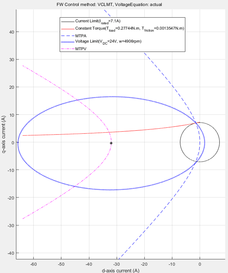
Figure 16: Constraint curves of a PMSM drawn at base speed (corner speed) and at rated torque.

Figure 17: Zoomed in portion of figure 16 to show the intersection of MTPA curve, current limit circle, and voltage limit curve.

Figure 18: The speed-torque characteristics of a PMSM that is marked at corner speed at rated torque.

You can use the following code to find the corner speed of the PMSM:

pmsm=mcb_SetPMSMMotorParameters('Teknic2310P');
pmsm.Rs=0.01;
pmsm.Lq=pmsm.Ld*2;
inverter=mcb_SetInverterParameters('BoostXL-DRV8305');
mcbPMSMSpeeds(pmsm,inverter,verbose=1);

Proceeding with the motorType as 'ipmsm'.
Corner speed [rpm] is: 4905.
Maximum speed [rpm] with VCLMT Field Weakening is: 6648.

Identifying Operating Points (id,iq)

For a given speed and load torque, you can find the operating points of a machine. The following sections explain the five selected operating points.

Case 1: MTPA Region of Operation

MTPA stands for Maximum Torque Per Ampere. A motor operates in MTPA region when $v_{s} = \sqrt{(v_{d}^{2} + v_{q}^{2})}$ is less than v_max.

To compute the optimal operating point, you can draw the constraint curves for the given speed and torque conditions.

Figure 19: Constraint curves of a PMSM drawn at a torque of 0.1N.m. and at a speed of 5000rpm. The corner speed at the given torque is higher than the given speed resulting in the possibility of MTPA operation.

Figure 20: Zoomed-in portion of the figure 19 to show the selected operating point for the given speed and torque.

Any point along the portion of the constant torque curve (between the marked points 1 and 2) that is within the region of overlap between the voltage limit ellipse and current limit circle results in the same torque output, while satisfying the voltage and current constraints. Point 1 results in the lowest current magnitude, and therefore, it is an optimal point of operation, which satisfies the voltage limit constraint and current limit constraint. In addition, this point meets the load torque demand and speed requirement.

Figure 21 (a): Drive characteristics of a PMSM that shows the speed and torque points.

Figure 21 (b): Current curves of the PMSM for the loaded torque that shows the operating point.

From the constraint curves shown in figure 20, you can notice that for the given speed, the voltage limit ellipse does not touch the operating point (id, iq), but encloses it. At a slightly higher speed (until the voltage limit curve touches the identified operating point) the same operating point (id, iq) is still the optimal operating point. Note that when the voltage limit curve touches the identified operating point (id, iq), $v_{s}$ becomes identical to $v_{\max}$ , and the corresponding speed is equal to the corner speed at the load torque. At a speed higher than this corner speed, you exceed the voltage limit if you follow the MTPA trajectory, and therefore, you can start the field weakening (FW) operation.

You can use the following code to plot the figures.

pmsm=mcb_SetPMSMMotorParameters('Teknic2310P');
pmsm.Rs=0.01;
pmsm.Lq=pmsm.Ld*2;
inverter=mcb_SetInverterParameters('BoostXL-DRV8305');
mcbPMSMCharacteristics(pmsm,inverter,torque=0.1,speed=5000,driveCharacteristics=0);

$Figure Constraint Curves of Teknic-2310P contains an axes object and another object of type subplottext. The axes object with xlabel d-axis current (A), ylabel q-axis current (A) contains 6 objects of type line. One or more of the lines displays its values using only markers These objects represent Current Limit(I_{rated}=7.1A), Constant Torque(T_{load}=0.1N.m, T_{friction}=0.0013807N.m), MTPA, Voltage Limit(V_{DC}=24V, w=5000rpm), MTPV.$

Case 2: Field-Weakening, Load Torque Lower Than Maximum Possible Torque at Given Speed

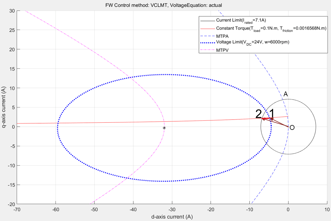
Figure 22: Constraint curve of the PMSM drawn at 0.1N.m. load torque at 6000 rpm with the constant torque curve passing through the intersection between current limit circle and voltage limit curve.

When you operate the motor at a speed higher than the corner speed along the MTPA trajectory, you exceed the voltage limit. Then the operating point moves along the constant torque curve to maintain the load torque demand. In figure 22, the constant torque curve passes through the intersection region of voltage limit curve and the current limit circle. This indicates that the when (id, iq) values are selected along the constant torque curve within this overlapping region, the system meets the load demand. However, the extremes of the possible points are marked 1 and 2 in the figure. Point 1 results in the lowest current magnitude, and therefore, the most optimal point for operation while satisfying the voltage limit constraint and the current limit constraint. It also meets the load torque demand and the speed requirement.

Figure 23: Zoomed-in portion of figure 22 that shows the selected operating point for optimal operation.

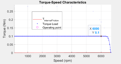
Figure 24 (a): Drive characteristics of a PMSM with the speed and torque point marked.

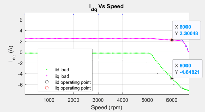
Figure 24 (b): Current curves of the PMSM for the loaded torque, with the operating point marked on them.

You can use the following code to plot the figures.

pmsm=mcb_SetPMSMMotorParameters('Teknic2310P');
pmsm.Rs=0.01;
pmsm.Lq=pmsm.Ld*2;
inverter=mcb_SetInverterParameters('BoostXL-DRV8305');
data=mcbPMSMCharacteristics(pmsm,inverter,torque=0.1,speed=6000,driveCharacteristics=0);

$Figure Constraint Curves of Teknic-2310P contains an axes object and another object of type subplottext. The axes object with xlabel d-axis current (A), ylabel q-axis current (A) contains 6 objects of type line. One or more of the lines displays its values using only markers These objects represent Current Limit(I_{rated}=7.1A), Constant Torque(T_{load}=0.1N.m, T_{friction}=0.0016568N.m), MTPA, Voltage Limit(V_{DC}=24V, w=6000rpm), MTPV.$

Case 3: Field-Weakening, Load Torque More Than Maximum Possible Torque at Given Speed

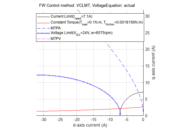
Figure 25: Constraint curves of the PMSM drawn at 0.1 N.m. and 6000 rpm speed with the constant torque curve not passing through the intersection of current limit circle and voltage limit curve.

Figure 25 shows a situation when the demand torque is higher than the possible torque at the given speed. In the figure, observe that the constant torque curve does not pass though the intersection region. Any point on the constant torque curve does not satisfy the current and voltage constraints. Therefore, only the maximum possible torque is returned as the operating point. This point is marked as 1 in the preceding figure.

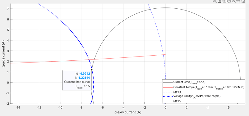
Figure 26: Zoomed-in portion of figure 25 showing the selected operating point.

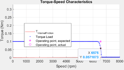
Figure 27 (a): Drive characteristics of a PMSM showing the speed and torque point.

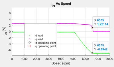
Figure 27 (b): Current curves of the PMSM for the loaded torque showing the operating point.

You can use the following code to plot the figures.

pmsm=mcb_SetPMSMMotorParameters('Teknic2310P');
pmsm.Rs=0.01;
pmsm.Lq=pmsm.Ld*2;
inverter=mcb_SetInverterParameters('BoostXL-DRV8305');
mcbPMSMCharacteristics(pmsm,inverter,torque=0.1,speed=6575,driveCharacteristics=0);

$Figure Constraint Curves of Teknic-2310P contains an axes object and another object of type subplottext. The axes object with xlabel d-axis current (A), ylabel q-axis current (A) contains 6 objects of type line. One or more of the lines displays its values using only markers These objects represent Current Limit(I_{rated}=7.1A), Constant Torque(T_{load}=0.1N.m, T_{friction}=0.0018156N.m), MTPA, Voltage Limit(V_{DC}=24V, w=6575rpm), MTPV.$

Case 4: MTPV, Load Torque Less Than Maximum Possible Torque at Given Speed

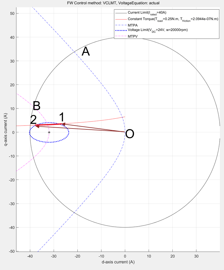
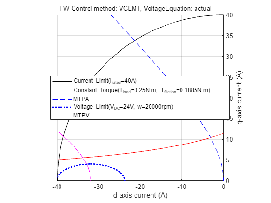
Figure 28: Constraint curves of a PMSM (designed to include MTPV region of operation) drawn at 0.25 N.m load and 20000 rpm speed with the constant torque curve passing through the intersection of current limit circle and voltage limit curve.

You can design a motor to have a possible MTPV operating region, by selecting a weaker magnet or by having a high current limit, or a combination of both. For motors that have a possible MTPV operating region, the constraint curves are drawn in the preceding figure. For these motors, theoretical speed limit is infinite, however, the practical maximum achievable speed of these motors is limited by the frictional load.

For these motors, field weakening operation begins after the MTPA region of operation. Beyond a specific speed of operation, which can be called the MTPV initiation speed, the voltage ellipse shrinks further. At higher speeds, it converges approximately at the critical current point. To satisfy the load torque, you can pick any point along the constant torque curve, which also satisfies the voltage constraint and current constraints. In other words, a point which lies within the intersection region of the current limit curve and the voltage limit curve.

The figure 28 shows a case where the demand load torque is lower than a torque that the motor can provide at the operating speed. For such operation, the points 1 and 2 are marked as the extremes of the possible points along the constant torque curve that satisfy the voltage and current constraints. The point 1 has the lowest current magnitude, making it the optimal point of operation.

Figure 29: Zoomed-in portion of figure 28 showing the selected operating point.

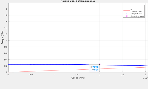
Figure 30 (a): Drive characteristics of a PMSM showing the speed and torque point.

Figure 30 (b): Current curves of the PMSM for the loaded torque showing the operating point.

You can use the following code to plot the figures.

pmsm=mcb_SetPMSMMotorParameters('Teknic2310P');
pmsm.Rs=0.01;
pmsm.I_rated=40;
pmsm.B=9e-5;
pmsm.Lq=pmsm.Ld*2;
inverter=mcb_SetInverterParameters('BoostXL-DRV8305');
mcbPMSMCharacteristics(pmsm,inverter,torque=0.25,speed=20000,driveCharacteristics=0);

$Figure Constraint Curves of Teknic-2310P contains an axes object and another object of type subplottext. The axes object with xlabel d-axis current (A), ylabel q-axis current (A) contains 6 objects of type line. One or more of the lines displays its values using only markers These objects represent Current Limit(I_{rated}=40A), Constant Torque(T_{load}=0.25N.m, T_{friction}=0.1885N.m), MTPA, Voltage Limit(V_{DC}=24V, w=20000rpm), MTPV.$

Case 5: MTPV, Load Torque More Than Maximum Possible Torque at Given Speed

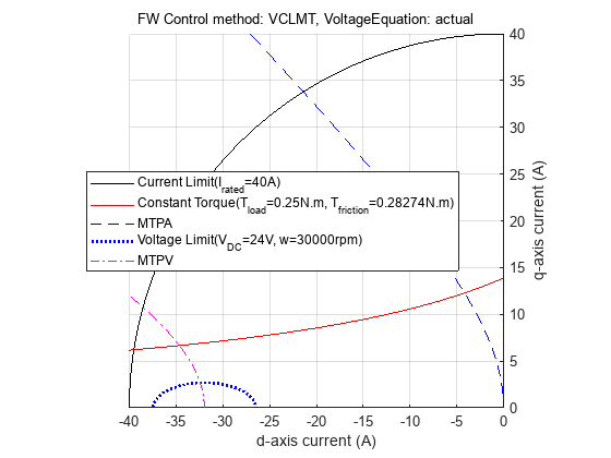
Figure 31: Constraint curve of a PMSM (designed to have MTPV region of operation) drawn at 0.25 N.m load and 30000 rpm speed with the constant torque curve not passing through the intersection of current limit circle and voltage limit curve.

Sometimes, the load torque can be higher than the torque that the motor can provide at the operating speed. In the preceding figure, this is represented by the constant torque curve not passing through the intersection of the current limit curve and voltage limit curve. Under this condition, the maximum torque is picked from the voltage limit curve. This is the point along the MTPV curve intersecting the voltage limit curve.

Figure 32: Zoomed-in portion of the figure 31 showing the selected operating point for optimal operation.

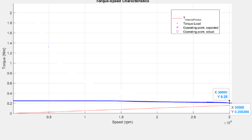
Figure 33 (a): Drive characteristics of a PMSM with the speed and torque point marked.

Figure 33 (b): Current curves of the PMSM for the loaded torque, with the operating point marked on them.

The preceding figure shows the selected operating point with circles. In addition, the figure also shows the speed-torque plot with the expected torque point, which is higher than the possible torque at that speed.

pmsm=mcb_SetPMSMMotorParameters('Teknic2310P');
pmsm.Rs=0.01;
pmsm.I_rated=40;
pmsm.B=9e-5;
pmsm.Lq=pmsm.Ld*2;
inverter=mcb_SetInverterParameters('BoostXL-DRV8305');
mcbPMSMCharacteristics(pmsm,inverter,torque=0.25,speed=30000,driveCharacteristics=0);

$Figure Constraint Curves of Teknic-2310P contains an axes object and another object of type subplottext. The axes object with xlabel d-axis current (A), ylabel q-axis current (A) contains 6 objects of type line. One or more of the lines displays its values using only markers These objects represent Current Limit(I_{rated}=40A), Constant Torque(T_{load}=0.25N.m, T_{friction}=0.28274N.m), MTPA, Voltage Limit(V_{DC}=24V, w=30000rpm), MTPV.$

Identifying Possible (MTPA-Field Weakening-MTPV) Control Currents

The preceding section showed that for different speeds and torques, optimal (id, iq) values can be derived.

In a typical motor control application, you need a reference current value for the operating speed and reference torque. Such reference currents can be derived using the preceding methods, which result in optimal operations.

LUT based PMSM Control Reference

The block LUT based PMSM Control Reference computes the id and iq look-up tables using the given motor parameters (either linear lumped parameters, or non-linear parameter maps) or uses the user-provided id, iq look-up table values.

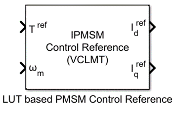
Figure 34 (a): LUT based PMSM Control Reference block, available in Motor Control Blockset library.

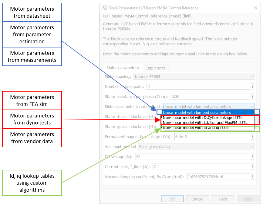
Figure 34 (b): The mask view for the block with options showing the input possibilities of motor parameters.

The LUT based PMSM Control reference block accepts multiple types of inputs that can utilize the externally generated (id, iq) LUTs or calculate the LUT based on the provided motor parameters (linear or non-linear). When you select the motor parameters (either linear or non-linear) as the parameter input method, the LUT based PMSM Control Reference block computes the LUTs on the host before the simulation begins or before the code-generation step.

mcbGenerateTables

You can use the function mcbGenerateTables available in Motor Control Blockset to create the id and iq LUTs on the host for custom grid sizes and grid point densities. The LUT based PMSM Control Reference block uses this function to compute the id and iq LUTs using the given motor parameters.

When the id and iq LUTs are generated, you can plot them in the d-q current space for multiple speed and torque values. When the point grid overlaps with the constraint curves of the motor, you can obtain figure 36. In the figure, the dots at the intersection of the curves are only for representation purposes. The output figure window of the function has segments of voltage limit curve and constant torque curves that are drawn within the current limit circle.

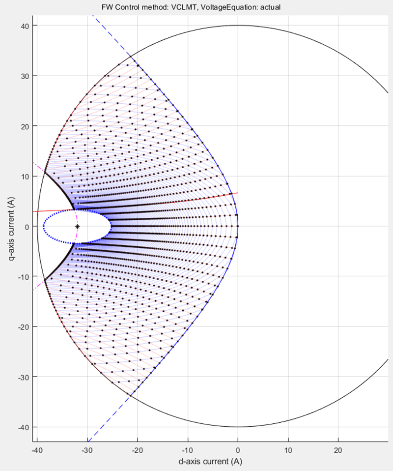
Figure 35 (a): Constraint curves of a PMSM (designed to have MTPV operating region) overlapped with the grid of (id, iq) Look-up Tables for different speeds and load torques.

Figure 35 (b): id LUT.

Figure 35 (c): iq LUT.

You can use the following code to create and plot a grid of id and iq with respect to speed and torque values.

pmsm=mcb_SetPMSMMotorParameters('Teknic2310P');
pmsm.Rs=0.01;
pmsm.I_rated=40;
pmsm.B=9e-5;
pmsm.Lq=pmsm.Ld*2;
inverter=mcb_SetInverterParameters('BoostXL-DRV8305');
seed.drawLUTonConstraintCurves=1;
seed.TBreakPointsCount=31;
seed.wBreakPointsCount=32;
PMSMLUT=mcbGenerateTables(pmsm,inverter,'idiqLUTs',seed);

$Figure Constraint Curves of Teknic-2310P contains an axes object and another object of type subplottext. The axes object with xlabel d-axis current (A), ylabel q-axis current (A) contains 101 objects of type line. These objects represent Current Limit(I_{rated}=40A), Constant Torque(T_{load}=0N.m, T_{friction}=0.2423N.m), MTPA, Voltage Limit(V_{DC}=24V, w=25708.3281rpm), MTPV.$

disp(PMSMLUT)

    drawLUTonConstraintCurves: 1
            TBreakPointsCount: 31
            wBreakPointsCount: 32
                        goLUT: 0
                    FWCMethod: 'vclmt'
                    motorType: 'ipmsm'
                      trefVec: [-2.1646 -2.0203 -1.8760 -1.7317 -1.5874 -1.4431 -1.2988 -1.1545 -1.0101 -0.8658 -0.7215 -0.5772 -0.4329 -0.2886 -0.1443 0 0.1443 0.2886 0.4329 0.5772 0.7215 0.8658 1.0101 1.1545 1.2988 1.4431 1.5874 … ] (1×31 double)
                      wrpmVec: [1 830 1660 2489 3318 4147 4977 5806 6635 7464 8294 9123 9952 10781 11611 12440 13269 14099 14928 15757 16586 17416 18245 19074 19903 20733 21562 22391 23221 24050 24879 25708]
                      idTable: [31×32 double]
                      iqTable: [31×32 double]

Simulation Using id, iq LUTs

Figure 36: View of Simulink model that is created to use the LUT based PMSM Control Reference block to generate [id, iq] reference values for a given load torque and a range of speed values. This model is used to create the (id, iq) reference values for the fractional rated torque values for the different speeds drawn, in the figures 21, 24, 27, 30, and 33.

You can observe that the LUT based PMSM Control Reference block can be used with a given load torque and a range of speed values to derive a possible speed-torque characteristic curve, similar to the ones shown in the figures in the earlier sections.

The following figures show the constraint curves of the motor that overlap with the data from the simulations using the LUT based PMSM Control Reference block.

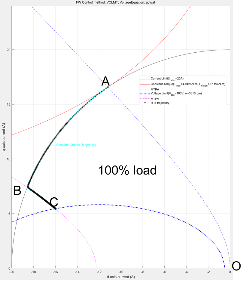
Figure 37 (a): Constraint curves of a PMSM drawn at envelope torque, showing the overlapped (id, iq) reference values generated from the LUT based PMSM Control Reference block.

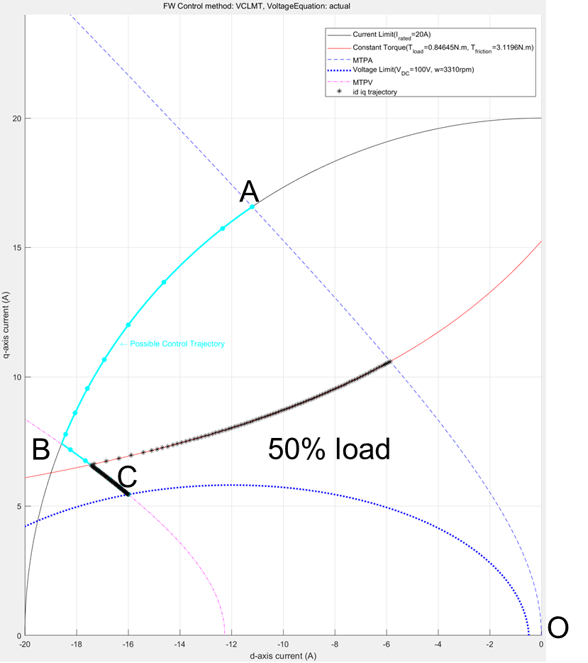
Figure 37 (b): Constraint curves of a PMSM drawn at half the rated torque, showing the overlapped [id, iq] reference values generated from the LUT based PMSM Control Reference block.

In the figures 37(a) and 37(b), notice that the black stars are the contour of points derived from the simulation that overlaps with the corresponding constraint curves. For both these cases, the MTPA region is not shown, because the torque demand begins from the maximum value and does not increase. For the case of 100% load, you can see that the operating points follow the field-weakening path along the current constraint curve and then the MTPV curve. For the case of 50%, you can see that the operating points follow the constant torque curve and then the MTPV curve.

An example mcb_pmsm_nonlin_fwc.slx uses the non-linear data from the FEA simulation software to demonstrate usage of non-linear motor parameters to derive the id, iq LUTs and derives the reference currents based on the operating conditions.

Figure 38: The example model mcb_pmsm_nonlin_fwc.slx.

PMSM Constraint Curves and Their Application

Required MathWorks Products

Fundamentals of Constraint Curves of PMSM

Current Limit Circle

Constant Torque Curve

MTPA Curve

Voltage Limit Curve

MTPV Curve

Using Constraint Curves

Find Maximum Operable Speed

Finding Corner Speed of Motor

Identifying Operating Points (id,iq)

Case 1: MTPA Region of Operation

Case 2: Field-Weakening, Load Torque Lower Than Maximum Possible Torque at Given Speed

Case 3: Field-Weakening, Load Torque More Than Maximum Possible Torque at Given Speed

Case 4: MTPV, Load Torque Less Than Maximum Possible Torque at Given Speed

Case 5: MTPV, Load Torque More Than Maximum Possible Torque at Given Speed

Identifying Possible (MTPA-Field Weakening-MTPV) Control Currents

LUT based PMSM Control Reference

mcbGenerateTables

Simulation Using id, iq LUTs

See Also