yregion
Description
yregion( creates one or more filled
regions between y-coordinates. To create one filled region, specify
y1,y2)y1 and y2 as scalars. To create multiple filled
regions, specify y1 and y2 as vectors of the same
length.
yregion( specifies the
target axes for the filled region. Specify ax,___)ax as the first argument in
any of the previous syntaxes.
yregion(___, specifies
properties for the region using one or more name-value arguments. If you create multiple
regions, the property values apply to all of the regions. For example, you can set the color
of a region to yellow by using Name=Value)yregion(5,10,FaceColor="yellow"). For a
list of properties, see ConstantRegion Properties.
yr = yregion(___) returns one or more
ConstantRegion objects. Use yr to set properties of
the filled regions after creating them. For a list of properties, see ConstantRegion Properties.
Examples
Create a line plot and a filled region between y=0 and y=106.
x = 0:0.1:50;
y = 2*x .* (sin(x) + cos(2*x));
plot(x,y)
yregion(0,106)

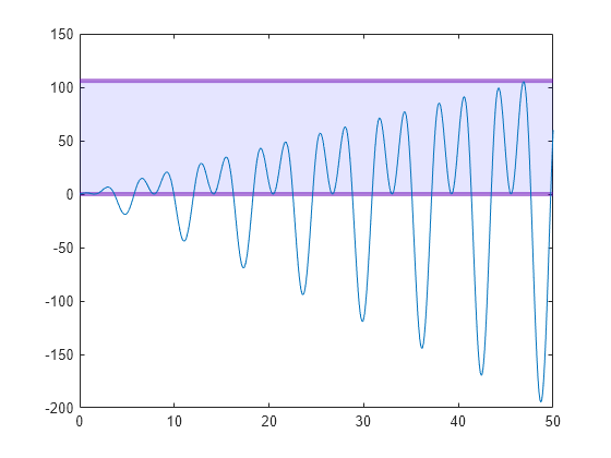
You can modify aspects of a region by setting properties. You can set properties by specifying name-value arguments when you call yregion, or you can set properties later using dot notation.
For example, create a plot with a filled region, and customize the fill and boundary line colors by specifying the FaceColor and EdgeColor name-value arguments. Also, specify an output argument to store the ConstantRegion object.
x = 0:0.1:50;
y = 2*x .* (sin(x) + cos(2*x));
plot(x,y)
yr = yregion(0,106,FaceColor="b",EdgeColor=[0.4 0 0.7]);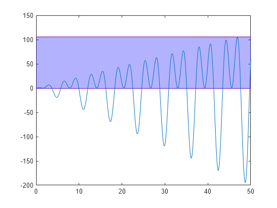
Modify the appearance further by setting properties of the ConstantRegion object yr. Change the opacity of the fill color and boundary line color by setting the FaceAlpha and EdgeAlpha properties to numbers from 0 to 1, where 1 is fully opaque. Then, set the boundary line thickness by setting the LineWidth property.
yr.FaceAlpha = 0.1;
yr.EdgeAlpha = 0.5;
yr.LineWidth = 3;
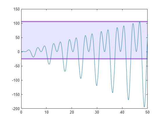
Move the lower boundary to -25.
yr.Value = [-25 106];
You can create multiple filled regions by specifying the starting and ending coordinates as vectors of the same size. You can also display entries for these regions in a legend.
For example, create a horizontal bar chart with two filled regions. Specify an output argument to store both ConstantRegion objects so you can modify them later.
x = [1 2 3 4 13 11 2.5];
barh(x,DisplayName="Results")
yr = yregion([0.5 4.5],[2.5 6.5]);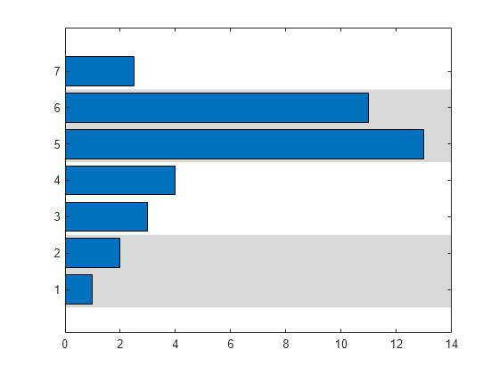
Specify a color for each region by setting the FaceColor property. Specify a legend entry name for each region by setting the DisplayName property. To access the individual ConstantRegion objects for setting the properties, index into the output argument yr. After setting the properties, display a legend.
yr(1).FaceColor = "r";
yr(1).DisplayName = "Low";
yr(2).FaceColor = "#88FE45";
yr(2).DisplayName = "High";
legend

Create a horizontal bar chart with five bars positioned at specific numbers of minutes. Then display a filled region from the second bar to the fourth bar. To contain the three bars within the region, calculate the boundaries by subtracting 30 seconds from the second bar's location and adding 30 seconds to the fourth bar's location.
dur = minutes(1:5)';
y = [1 5 11 4 3];
barh(dur,y)
yregion(dur(2)-seconds(30), dur(4)+seconds(30))

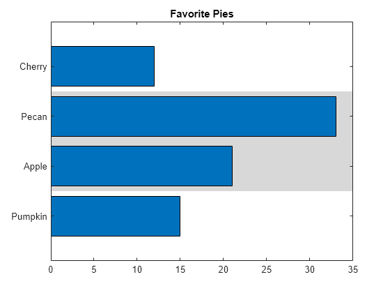
Create a horizontal bar chart of categorical data, and create a filled region that spans the second and third bars. The reordercats function specifies the order of the categories for the bar chart.
cats = categorical(["Pumpkin" "Apple" "Pecan" "Cherry"]);
cats = reordercats(cats,["Pumpkin" "Apple" "Pecan" "Cherry"]);
barlengths = [15 21 33 12];
barh(cats,barlengths)
yregion(cats(2),cats(3))
title("Favorite Pies")
Since R2023b
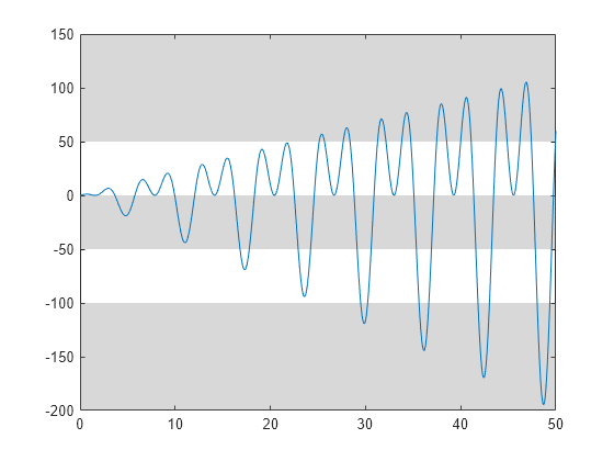
Create a plot, and add three filled regions. Specify a 2-by-3 matrix with the lower bounds in the first row and the upper bounds in the second row. The first region has a lower bound of -Inf, and the last region has an upper bound of Inf, so the first and last regions are unbounded.
x = 0:0.1:50;
y = 2*x .* (sin(x) + cos(2*x));
plot(x,y)
Y = [-Inf -50 50; -100 0 Inf];
yregion(Y)
Input Arguments
Name-Value Arguments
Specify optional pairs of arguments as
Name1=Value1,...,NameN=ValueN, where Name is
the argument name and Value is the corresponding value.
Name-value arguments must appear after other arguments, but the order of the
pairs does not matter.
Example: yregion(5,10,FaceColor="yellow") creates a yellow filled
region.
Note
The properties listed here are only a subset. For a complete list, see ConstantRegion Properties.
Fill color, specified as an RGB triplet, a hexadecimal color code, or a color name.
For a custom color, specify an RGB triplet or a hexadecimal color code.
An RGB triplet is a three-element row vector whose elements specify the intensities of the red, green, and blue components of the color. The intensities must be in the range
[0,1], for example,[0.4 0.6 0.7].A hexadecimal color code is a string scalar or character vector that starts with a hash symbol (
#) followed by three or six hexadecimal digits, which can range from0toF. The values are not case sensitive. Therefore, the color codes"#FF8800","#ff8800","#F80", and"#f80"are equivalent.
Alternatively, you can specify some common colors by name. This table lists the named color options, the equivalent RGB triplets, and the hexadecimal color codes.
| Color Name | Short Name | RGB Triplet | Hexadecimal Color Code | Appearance |
|---|---|---|---|---|
"red" | "r" | [1 0 0] | "#FF0000" |
|
"green" | "g" | [0 1 0] | "#00FF00" |
|
"blue" | "b" | [0 0 1] | "#0000FF" |
|
"cyan"
| "c" | [0 1 1] | "#00FFFF" |
|
"magenta" | "m" | [1 0 1] | "#FF00FF" |
|
"yellow" | "y" | [1 1 0] | "#FFFF00" |
|
"black" | "k" | [0 0 0] | "#000000" |
|
"white" | "w" | [1 1 1] | "#FFFFFF" |
|
"none" | Not applicable | Not applicable | Not applicable | No color |
This table lists the default color palettes for plots in the light and dark themes.
| Palette | Palette Colors |
|---|---|
Before R2025a: Most plots use these colors by default. |
|
|
|
You can get the RGB triplets and hexadecimal color codes for these palettes using the orderedcolors and rgb2hex functions. For example, get the RGB triplets for the "gem" palette and convert them to hexadecimal color codes.
RGB = orderedcolors("gem");
H = rgb2hex(RGB);
Before R2023b: Get the RGB triplets using RGB =
get(groot,"FactoryAxesColorOrder").
Before R2024a: Get the hexadecimal color codes using H =
compose("#%02X%02X%02X",round(RGB*255)).
Boundary line color, specified as an RGB triplet, a hexadecimal color code, or a color name.
For a custom color, specify an RGB triplet or a hexadecimal color code.
An RGB triplet is a three-element row vector whose elements specify the intensities of the red, green, and blue components of the color. The intensities must be in the range
[0,1], for example,[0.4 0.6 0.7].A hexadecimal color code is a string scalar or character vector that starts with a hash symbol (
#) followed by three or six hexadecimal digits, which can range from0toF. The values are not case sensitive. Therefore, the color codes"#FF8800","#ff8800","#F80", and"#f80"are equivalent.
Alternatively, you can specify some common colors by name. This table lists the named color options, the equivalent RGB triplets, and the hexadecimal color codes.
| Color Name | Short Name | RGB Triplet | Hexadecimal Color Code | Appearance |
|---|---|---|---|---|
"red" | "r" | [1 0 0] | "#FF0000" |
|
"green" | "g" | [0 1 0] | "#00FF00" |
|
"blue" | "b" | [0 0 1] | "#0000FF" |
|
"cyan"
| "c" | [0 1 1] | "#00FFFF" |
|
"magenta" | "m" | [1 0 1] | "#FF00FF" |
|
"yellow" | "y" | [1 1 0] | "#FFFF00" |
|
"black" | "k" | [0 0 0] | "#000000" |
|
"white" | "w" | [1 1 1] | "#FFFFFF" |
|
"none" | Not applicable | Not applicable | Not applicable | No color |
This table lists the default color palettes for plots in the light and dark themes.
| Palette | Palette Colors |
|---|---|
Before R2025a: Most plots use these colors by default. |
|
|
|
You can get the RGB triplets and hexadecimal color codes for these palettes using the orderedcolors and rgb2hex functions. For example, get the RGB triplets for the "gem" palette and convert them to hexadecimal color codes.
RGB = orderedcolors("gem");
H = rgb2hex(RGB);
Before R2023b: Get the RGB triplets using RGB =
get(groot,"FactoryAxesColorOrder").
Before R2024a: Get the hexadecimal color codes using H =
compose("#%02X%02X%02X",round(RGB*255)).
Fill color transparency, specified as a scalar in the range [0,1]. A value of 1 is opaque and 0 is completely transparent. Values between 0 and 1 are partially transparent.
Boundary line transparency, specified as a scalar in the range [0,1]. A value of 1 is opaque and 0 is completely transparent. Values between 0 and 1 are partially transparent.
Boundary line style, specified as one of the options listed in this table.
| Line Style | Description | Resulting Line |
|---|---|---|
"-" | Solid line |
|
"--" | Dashed line |
|
":" | Dotted line |
|
"-." | Dash-dotted line |
|
"none" | No line | No line |