centrality
Measure node importance
Description
C = centrality(___,Name,Value)centrality(G,'closeness','Cost',c) specifies the cost of
traversing each edge.
Examples
Create and plot a graph containing six fictitious websites.
s = [1 1 2 2 3 3 3 4 5];
t = [2 5 3 4 4 5 6 1 1];
names = {'http://www.example.com/alpha', 'http://www.example.com/beta', ...
         'http://www.example.com/gamma', 'http://www.example.com/delta', ...
         'http://www.example.com/epsilon', 'http://www.example.com/zeta'};
G = digraph(s,t,[],names);
plot(G,'NodeLabel',{'alpha','beta','gamma','delta','epsilon','zeta'})
Calculate the page rank of each website using the centrality function. Append this information to the Nodes table of the graph as an attribute of the graph nodes.
pg_ranks = centrality(G,'pagerank')pg_ranks = 6×1
0.3210
0.1706
0.1066
0.1368
0.2008
0.0643
G.Nodes.PageRank = pg_ranks;
G.Nodes
ans=6×2 table
                   Name                   PageRank
    __________________________________    ________

    {'http://www.example.com/alpha'  }    0.32098
    {'http://www.example.com/beta'   }    0.17057
    {'http://www.example.com/gamma'  }    0.10657
    {'http://www.example.com/delta'  }    0.13678
    {'http://www.example.com/epsilon'}    0.20078
    {'http://www.example.com/zeta'   }    0.06432
Also determine which nodes are hubs and authorities using centrality and append the scores to the Nodes table.
hub_ranks = centrality(G,'hubs');
auth_ranks = centrality(G,'authorities');
G.Nodes.Hubs = hub_ranks;
G.Nodes.Authorities = auth_ranks;
G.Nodes
ans=6×4 table
                   Name                   PageRank       Hubs       Authorities
    __________________________________    ________    __________    ___________

    {'http://www.example.com/alpha'  }    0.32098        0.24995    7.3237e-05
    {'http://www.example.com/beta'   }    0.17057        0.24995      0.099993
    {'http://www.example.com/gamma'  }    0.10657        0.49991      0.099993
    {'http://www.example.com/delta'  }    0.13678     9.1536e-05       0.29998
    {'http://www.example.com/epsilon'}    0.20078     9.1536e-05       0.29998
    {'http://www.example.com/zeta'   }    0.06432              0       0.19999
Create and plot a weighted graph using a random sparse adjacency matrix. Since there are a lot of edges, use a very small value for EdgeAlpha to make the edges mostly transparent.
A = sprand(1000,1000,0.15);
A = A + A';
G = graph(A,'omitselfloops');
p = plot(G,'Layout','force','EdgeAlpha',0.005,'NodeColor','r');

Calculate the degree centrality of each node. Specify the importance of each edge using the edge weights.
deg_ranks = centrality(G,'degree','Importance',G.Edges.Weight);
Use discretize to place the nodes into 7 equally-spaced bins based on their centrality scores.
edges = linspace(min(deg_ranks),max(deg_ranks),7);
bins = discretize(deg_ranks,edges);
Make the size of each node in the plot proportional to its centrality score. The marker size of each node is equal to the bin number (1-7).
p.MarkerSize = bins;

Load the data in minnesota.mat, which contains a graph object G representing the network of roads in Minnesota. The graph nodes have xy coordinates contained in the XCoord and YCoord variables of the G.Nodes table.
load minnesota.mat
xy = [G.Nodes.XCoord G.Nodes.YCoord];
Add edge weights to the graph that roughly correspond to the length of the roads, calculated using the Euclidean distance between the xy coordinates of the end nodes of each edge.
[s,t] = findedge(G);
G.Edges.Weight = hypot(xy(s,1)-xy(t,1), xy(s,2)-xy(t,2));
Plot the graph using the xy coordinates for the nodes.
p = plot(G,'XData',xy(:,1),'YData',xy(:,2),'MarkerSize',5);
title('Minnesota Road Network')

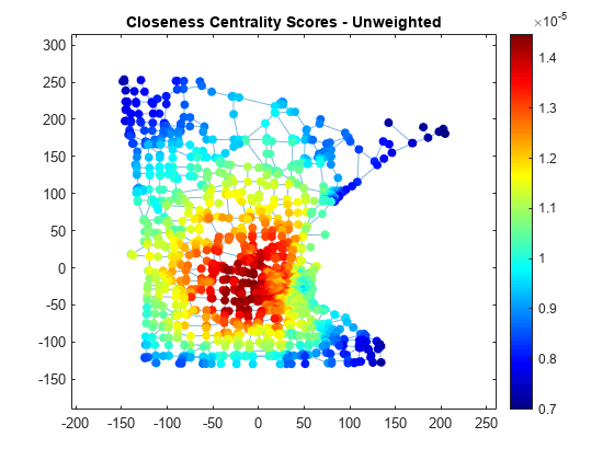
Compute the closeness centrality of each node. Scale the node color NodeCData to be proportional to the centrality score.
ucc = centrality(G,'closeness');
p.NodeCData = ucc;
colormap jet
colorbar
title('Closeness Centrality Scores - Unweighted')

Also compute the weighted closeness centrality score, using the edge weights as the cost of traversing each edge. Using the road lengths as edge weights improves the score quality, since distances are now measured as the sum of the lengths of all traveled edges, rather than the number of edges traveled.
wcc = centrality(G,'closeness','Cost',G.Edges.Weight);
p.NodeCData = wcc;
title('Closeness Centrality Scores - Weighted')

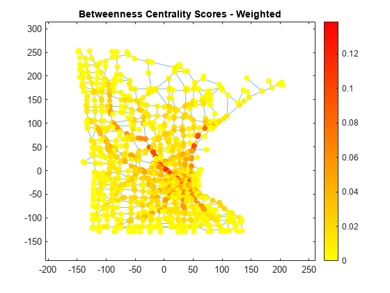
Compute the weighted betweenness centrality scores for the graph to determine the roads most often found on the shortest path between two nodes. Normalize the centrality scores with the factor so that the score represents the probability that a traveler along a shortest path between two random nodes will travel through a given node. The plot indicates that there are a few very important roads leading into and out of the city.
wbc = centrality(G,'betweenness','Cost',G.Edges.Weight);
n = numnodes(G);
p.NodeCData = 2*wbc./((n-2)*(n-1));
colormap(flip(autumn,1));
title('Betweenness Centrality Scores - Weighted')

Input Arguments
Type of node centrality, specified as one of the options in the table. The table also lists the compatible name-value arguments that work with each type. Each variety of node centrality offers a different measure of node importance in a graph.
|
Option |
Graph type |
Description | Name-Value Arguments |
|---|---|---|---|
|
|
Undirected | The
If you specify | |
|
|
Directed | ||
|
|
Undirected |
The Ai is the
number of reachable nodes from node
| |
|
|
Directed | ||
|
|
Undirected or Directed |
The is the number of shortest paths from
| |
|
|
Undirected or Directed | The
| |
|
|
Undirected |
The
| |
|
|
Directed |
The
|
Note
The centrality function assumes all edge weights
are equal to 1. To change this, specify edge weights for use with the
'Cost' or 'Importance'
name-value pairs.
Example: centrality(G,'degree')
Example: centrality(G,'hubs','Tolerance',tol)
Name-Value Arguments
Specify optional pairs of arguments as
Name1=Value1,...,NameN=ValueN, where Name is
the argument name and Value is the corresponding value.
Name-value arguments must appear after other arguments, but the order of the
pairs does not matter.
Before R2021a, use commas to separate each name and value, and enclose
Name in quotes.
Example: C = centrality(G,'closeness','Cost',edgeCosts) computes
the closeness centrality using edgeCosts as the cost (weight) of
traversing each edge in the graph.
Cost of edge traversal, specified as the comma-separated pair
consisting of 'Cost' and a vector of edge weights.
The ith edge weight specifies the cost associated with traversing the
edge findedge(G,i).
For the
'closeness','outcloseness', and'incloseness'centrality types, edge costs must be nonnegative.For the
'betweenness'centrality type, edge costs must be positive.
'Cost' edge weights are smaller when the connection
is shorter, or faster, or cheaper. Some examples of
'Cost' edge weights are:
Length of a path
Travel time
Cost of a ticket
Note
'Cost' only applies to the
'closeness',
'outcloseness',
'incloseness', and
'betweenness' centrality types.
Example: centrality(G,'closeness','Cost',c)
Probability of selecting a successor node, specified as the
comma-separated pair consisting of
'FollowProbability' and a scalar between 0 and 1.
The follow probability is the probability that the next node selected in
the traversal by the pagerank algorithm is chosen among the successors
of the current node, and not at random from all nodes. For websites,
this probability corresponds to clicking a link on the current web page
instead of surfing to another random web page.
Note
'FollowProbability' only applies to the
'pagerank' centrality type.
Example: centrality(G,'pagerank','FollowProbability',0.5)
Edge importance, specified as the comma-separated pair consisting of
'Importance' and a vector of nonnegative edge
weights. The ith edge weight specifies the importance of the edge
findedge(G,i). An edge weight of zero is
equivalent to removing that edge from the graph.
For multigraphs with multiple edges between two nodes,
centrality adds the multiple edges together and
treats them as a single edge with the combined weight.
'Importance' edge weights are larger when the
connection is stronger. Some examples of 'Importance'
edge weights are:
Number of travellers per day
Number of clicks on a link
Number of papers published together
Note
'Importance' only applies to the
'degree', 'outdegree',
'indegree', 'pagerank',
'eigenvector', 'hubs', and
'authorities' centrality types.
Example: centrality(G,'degree','Importance',x)
Maximum number of iterations, specified as the comma-separated pair
consisting of 'MaxIterations' and a scalar. The
centrality algorithm runs until the tolerance
is met or the maximum number of iterations is reached, whichever comes
first.
Note
'MaxIterations' only applies to the
'pagerank', 'eigenvector',
'hubs', and 'authorities'
centrality types.
Example: centrality(G,'pagerank','MaxIterations',250)
Stopping criterion for iterative solvers, specified as the
comma-separated pair consisting of 'Tolerance' and a
scalar. The centrality algorithm runs until the
tolerance is met or the maximum number of iterations is reached,
whichever comes first.
Note
'Tolerance' only applies to the
'pagerank', 'eigenvector',
'hubs', and 'authorities'
centrality types.
Example: centrality(G,'pagerank','Tolerance',1e-5)
Output Arguments
Node centrality scores, returned as a column vector.
C(i) is the centrality score of node
i. The interpretation of the node centrality score
depends on the type of centrality computation selected. The more central a
node is, the larger its centrality score.
Extended Capabilities
Thread-Based Environment
Run code in the background using MATLAB® backgroundPool or accelerate code with Parallel Computing Toolbox™ ThreadPool.
Version History
Introduced in R2016a
MATLAB Command
You clicked a link that corresponds to this MATLAB command:
Run the command by entering it in the MATLAB Command Window. Web browsers do not support MATLAB commands.
Select a Web Site
Choose a web site to get translated content where available and see local events and offers. Based on your location, we recommend that you select: .
You can also select a web site from the following list
How to Get Best Site Performance
Select the China site (in Chinese or English) for best site performance. Other MathWorks country sites are not optimized for visits from your location.
Americas
- América Latina (Español)
- Canada (English)
- United States (English)
Europe
- Belgium (English)
- Denmark (English)
- Deutschland (Deutsch)
- España (Español)
- Finland (English)
- France (Français)
- Ireland (English)
- Italia (Italiano)
- Luxembourg (English)
- Netherlands (English)
- Norway (English)
- Österreich (Deutsch)
- Portugal (English)
- Sweden (English)
- Switzerland
- United Kingdom (English)