geoscatter

R2026b

Scatter chart in geographic coordinates

• 

Syntax

geoscatter(lat,lon)

geoscatter(lat,lon,A)

geoscatter(lat,lon,A,C)

geoscatter(___,"filled")

geoscatter(___,mkr)

geoscatter(tbl,latvar,lonvar)

geoscatter(tbl,latvar,lonvar,"filled")

geoscatter(ax,___)

geoscatter(___,Name,Value)

s = geoscatter(___)

Description

Vector and Matrix Data

geoscatter(lat,lon) creates a scatter plot with markers in geographic coordinates. By default, the function uses circular markers. Specify the latitude coordinates in degrees using lat, and specify the longitude coordinates in degrees using lon.

• To plot one set of coordinates, specify lat and lon as vectors of the same length.

• To plot multiple sets of coordinates on the same set of axes, specify at least one of lat or lon as a matrix. (since R2026b)

If the current axes is not a geographic or map axes, or if there is no current axes, then the function creates the scatter plot in a new geographic axes.

geoscatter(lat,lon,A) specifies the circle sizes in points squared. To use the same size for all the circles, specify A as a scalar. To plot each circle with a different size, specify A as a vector or a matrix.

geoscatter(lat,lon,A,C) specifies the circle colors. You can specify one color for all the circles, or you can vary the color. For example, you can plot all red circles by specifying C as "red".

geoscatter(___,"filled") fills in the circles. You can use the "filled" option with any of the input argument combinations in the previous syntaxes.

geoscatter(___,mkr) specifies the marker type.

Table Data

geoscatter(tbl,latvar,lonvar) plots the variables latvar and lonvar from the table tbl. To plot one data set, specify one variable for latvar and one variable for lonvar. To plot multiple data sets, specify multiple variables for latvar, lonvar, or both. If both arguments specify multiple variables, they must specify the same number of variables. (Since R2022b)

geoscatter(tbl,latvar,lonvar,"filled") plots the specified variables from the table with filled circles.

Additional Options

geoscatter(ax,___) plots into the geographic axes or map axes specified by ax. Specify the axes as the first argument in any of the previous syntaxes.

geoscatter(___,Name,Value) specifies properties of the scatter plot using one or more name-value arguments. For a list of properties, see Scatter Properties.

s = geoscatter(___) returns the Scatter object or a vector of Scatter objects. Use s to set properties after creating the plot. For a full list of properties, see Scatter Properties.

Examples

Create Geographic Scatter Plot

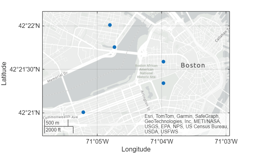
Specify the latitude and longitude coordinates of several locations in Boston. Create a scatter plot using filled markers.

lat = [42.3501 42.3598 42.3626 42.3668 42.3557];
lon = [-71.0870 -71.0662 -71.0789 -71.0801 -71.0662];
geoscatter(lat,lon,"filled")

Zoom out of the plot by adjusting the limits.

geolimits([42.3456 42.3694],[-71.0930 -71.0536])

Use Markers with Varying Sizes and Colors

Create a scatter plot using the latitude and longitude coordinates of several points along the Mississippi River. Specify the optional size and color arguments as vectors. The color values map to colors in the colormap.

lat = [32.30 33.92 35.17 36.98 37.69 38.34];
lon = [-91.05 -91.18 -90.09 -89.11 -89.52 -90.37];
A = 100*[5 12 15 3 10 3];
C = [1 2 2 3 1 1];

geoscatter(lat,lon,A,C,"filled")

Zoom out by adjusting the latitude and longitude limits of the plot. Then, change the basemap to a terrain basemap.

geolimits([31.60 38.91],[-97.04 -82.84])
geobasemap grayterrain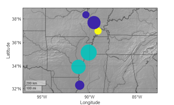

Specify Marker Symbol

Specify the latitude and longitude coordinates of several European cities. Create a scatter plot using magenta diamond markers.

lat = [48.85 51.5 40.41 41.9 52.52 52.36 52.22 47.49 44.42 50.07 48.20 46.94];
lon = [2.35 -0.12 -3.70 12.49 13.40 4.90 21.01 19.04 26.10 14.43 16.37 7.44];

geoscatter(lat,lon,"m","d")

Zoom out by adjusting the latitude and longitude limits of the plot. Then, change the basemap to a topographic basemap.

geolimits([30 60],[-20 50])
geobasemap topographic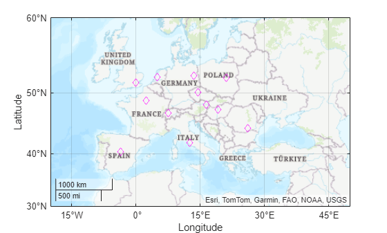

Change Marker Color and Line Width

Specify the latitude and longitude coordinates of several locations in Boston.

lat = [42.3501 42.3598 42.3626 42.3668 42.3557];
lon = [-71.0870 -71.0662 -71.0789 -71.0801 -71.0662];

Create a scatter plot and set the marker edge color, marker face color, and line width.

geoscatter(lat,lon,70,"MarkerEdgeColor",[0.9290 0.6940 0.1250], ...
    "MarkerFaceColor",[0.3010 0.7450 0.9330],"LineWidth",2)

Zoom out of the plot by adjusting the limits. Then, change the basemap.

geolimits([42.3456 42.3694],[-71.0930 -71.0536])
geobasemap streets-dark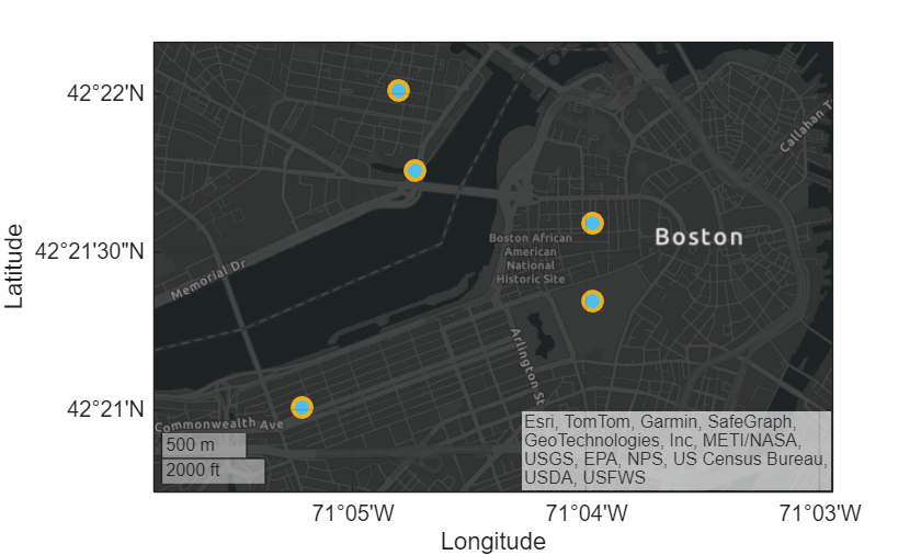

Plot Data from Table

Since R2022b

A convenient way to plot data from a table is to pass the table to the geoscatter function and specify the variables to plot.

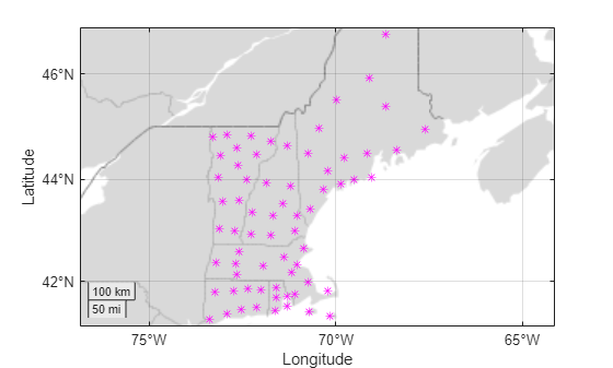
Load a file containing county data into the workspace as a table. The table includes latitude and longitude coordinates in the table variables Latitude and Longitude, respectively.

tbl = readtable("counties.xlsx"); 

Plot the latitude and longitude coordinates over a two-tone basemap. Return the Scatter object as s.

s = geoscatter(tbl,"Latitude","Longitude");
geobasemap grayland

Change the marker style and color of the plot by setting the Marker and MarkerEdgeColor properties.

s.Marker = "*";
s.MarkerEdgeColor = "m";

Plot Table Data with Custom Colors and Marker Sizes

Since R2022b

One way to plot data from a table and customize the colors and marker sizes is to set the ColorVariable and SizeData properties. You can set these properties as name-value arguments when you call the geoscatter function, or you can set them on the Scatter object later.

For example, load a file containing county data into the workspace as a table. The table includes latitude and longitude coordinates in the table variables Latitude and Longitude, respectively.

tbl = readtable("counties.xlsx");

Plot the latitude and longitude coordinates using filled markers. Return the Scatter object as s.

s = geoscatter(tbl,"Latitude","Longitude","filled");

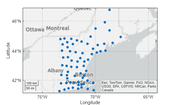
Change the marker sizes to 100 points by setting the SizeData property.

s.SizeData = 100;

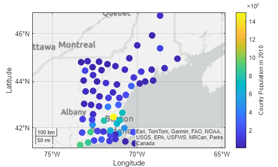
Vary the marker colors by setting the ColorVariable property to a table variable. Then, add a colorbar.

s.ColorVariable = "Population2010";
c = colorbar;
c.Label.String = "County Population in 2010";

Input Arguments

lat — Latitude coordinates in degrees

scalar | vector | matrix (since R2026b)

Latitude coordinates in degrees, specified as a scalar, vector, or matrix with elements in the range [–90, 90]. This argument can contain NaN values.

The size and shape of lat depends on the shape of your data. This table describes the most common situations.

Type of Plot	How to Specify Coordinates
One point	Specify lat and lon as scalars. For example: geoscatter(1,2)
One set of points	Specify lat and lon as any combination of row or column vectors of the same length. For example: geoscatter([1 2 3],[4; 5; 6])
Multiple sets of points that are different colors (since R2026b)	If all the sets share the same latitude or longitude coordinates, specify the shared coordinates as a vector and the other coordinates as a matrix. The length of the vector must match one of the dimensions of the matrix. For example: geoscatter([1 2 3],[4 5 6; 7 8 9]) If the matrix is square, the function plots a separate set of points for each column in the matrix. Alternatively, specify lat and lon as matrices of equal size. In this case, the function plots each column of lon against the corresponding column of lat. For example: geoscatter([1 2 3; 4 5 6],[7 8 9; 10 11 12])

Data Types: single | double

lon — Longitude coordinates in degrees

scalar | vector | matrix (since R2026b)

Longitude coordinates in degrees, specified as a scalar, vector, or matrix. This argument can contain NaN values.

The size and shape of lon depends on the shape of your data. This table describes the most common situations.

Type of Plot	How to Specify Coordinates
One point	Specify lat and lon as scalars. For example: geoscatter(1,2)
One set of points	Specify lat and lon as any combination of row or column vectors of the same length. For example: geoscatter([1 2 3],[4; 5; 6])
Multiple sets of points that are different colors (since R2026b)	If all the sets share the same latitude or longitude coordinates, specify the shared coordinates as a vector and the other coordinates as a matrix. The length of the vector must match one of the dimensions of the matrix. For example: geoscatter([1 2 3],[4 5 6; 7 8 9]) If the matrix is square, the function plots a separate set of points for each column in the matrix. Alternatively, specify lat and lon as matrices of equal size. In this case, the function plots each column of lon against the corresponding column of lat. For example: geoscatter([1 2 3; 4 5 6],[7 8 9; 10 11 12])

Data Types: single | double

A — Marker size, in points squared

36 (default) | numeric scalar | numeric vector | matrix (since R2026b) | []

Marker size with units in points squared, specified as a numeric scalar, vector, matrix, or empty array ([]). The size controls the area of each marker.

An empty array specifies the default size of 36 points. Use this option when you want to specify the color input argument and use the default marker area, such as geoscatter(lat,lon,[],C).

The way you specify the size depends on how you specify lat and lon, and how you want the plot to look. This table describes the most common situations.

Desired Marker Sizes	lat and lon	A	Example
Same size for all points	Any valid combination of vectors or matrices for lat and lon	Scalar	Specify lat as a vector, lon as a matrix, and A as a scalar. lat = [1 2 3 4]; lon = [1 6; 3 8; 2 7; 4 9]; geoscatter(lat,lon,100)
Different size for each point	Vectors of the same length	A vector with the same length as lat and lon. A matrix with at least one dimension that matches the lengths of lat and lon. Specifying a matrix is useful for displaying multiple markers with different sizes at each latitude-longitude location.	Specify lat, lon, and A as vectors. lat = [1 2 3 4]; lon = [1 3 2 4]; A = [80 150 700 50]; geoscatter(lat,lon,A) Specify lat and lon as vectors and A as a matrix. lat = [1 2 3 4]; lon = [1 3 2 4]; A = [80 30; 150 900; 50 2000; 200 350]; geoscatter(lat,lon,A)
Different size for each point	At least one of lat or lon is a matrix for plotting multiple data sets	A vector with the same number of elements as there are points in each data set. A matrix that has the same size as the lat or lon matrix.	Specify lat as a vector, lon as a matrix, and A as a vector. lat = [1 2 3 4]; lon = [1 6; 3 8; 2 7; 4 9]; A = [80 150 50 700]; geoscatter(lat,lon,A) Specify lat as a vector, lon as a matrix, and A as a matrix the same size as lon. lat = [1 2 3 4]; lon = [1 6; 3 8; 2 7; 4 9]; A = [80 30; 150 900; 50 2000; 200 350]; geoscatter(lat,lon,A)

The SizeData property of the scatter object stores the marker sizes.

C — Marker color

color name | RGB triplet | matrix of RGB triplets | vector of colormap indices

Marker color, specified as a color name, RGB triplet, matrix of RGB triplets, or a vector of colormap indices.

• Color name — A color name such as "red", or a short name such as "r".

• RGB triplet — A three-element row vector whose elements specify the intensities of the red, green, and blue components of the color. The intensities must be in the range [0,1]; for example, [0.4 0.6 0.7]. RGB triplets are useful for creating custom colors.

• Matrix of RGB triplets — A three-column matrix in which each row is an RGB triplet.

• Vector of colormap indices — A vector of numeric values that is the same length as the lat and lon vectors.

The way you specify the color depends on the desired color scheme and whether you are plotting one set of coordinates or multiple sets of coordinates. This table describes the most common situations.

Color Scheme	How to Specify the Color	Example
Use one color for all the points.	Specify a color name or a short name from the Color Names and RGB Triplets for Common Colors table, or specify one RGB triplet.	Plot one set of points, and specify the color as "red". geoscatter(1:4,[2 5 3 7],[],"red") Plot two sets of points, and specify the color as red using an RGB triplet. geoscatter(1:4,[2 5; 1 2; 8 4; 11 9],[],[1 0 0])
Assign different colors to each point using a colormap.	Specify a row or column vector of numbers. The numbers map into the current colormap array. The smallest value maps to the first row in the colormap, and the largest value maps to the last row. The intermediate values map linearly to the intermediate rows. If your plot has three points, specify a column vector to ensure the values are interpreted as colormap indices. You can use this method only when lat, lon, and A are all vectors.	Create a vector C that specifies four colormap indices. Plot four points using the colors from the current colormap. Then, change the colormap to winter. C = 1:4; geoscatter(1:4,[2 5 3 7],[],C) colormap(gca,"winter")
Create a custom color for each point.	Specify an m-by-3 matrix of RGB triplets, where m is the number of points in the plot.	Create a matrix C that specifies RGB triplets for green, red, gray, and purple. Then create a scatter plot of four points using those colors. C = [0 1 0; 1 0 0; 0.5 0.5 0.5; 0.6 0 1]; geoscatter(1:4,[2 5 3 7],[],C)
Create a different color for each data set.	Specify an n-by-3 matrix of RGB triplets, where n is the number of data sets. You can use this method only when at least one of lat, lon, or A is a matrix.	Create a matrix C that contains two RGB triplets. Then plot two data sets using those colors. C = [1 0 0; 0.6 0 1]; s = geoscatter(1:4,[2 5; 1 2; 8 4; 11 9],[],C)

Color Names and RGB Triplets for Common Colors

Color Name	Short Name	RGB Triplet	Appearance
"red"	"r"	[1 0 0]
"green"	"g"	[0 1 0]
"blue"	"b"	[0 0 1]
"cyan"	"c"	[0 1 1]
"magenta"	"m"	[1 0 1]
"yellow"	"y"	[1 1 0]
"black"	"k"	[0 0 0]
"white"	"w"	[1 1 1]

When you specify marker colors, the geoscatter function sets the MarkerFaceColor property of the Scatter object to "flat" and stores the marker colors in the CData property.

mkr — Marker symbol

"o" (default) | "+" | "*" | "." | "x" | ...

Marker symbol, specified as one of these values.

Marker	Description	Resulting Marker
"o"	Circle
"+"	Plus sign
"*"	Asterisk
"."	Point
"x"	Cross
"_"	Horizontal line
"|"	Vertical line
"square"	Square
"diamond"	Diamond
"^"	Upward-pointing triangle
"v"	Downward-pointing triangle
">"	Right-pointing triangle
"<"	Left-pointing triangle
"pentagram"	Pentagram
"hexagram"	Hexagram

"filled" — Option to fill the interior of the markers

"filled"

Option to fill the interior of the markers, specified as "filled". Use this option with markers that have a face, for example, "o" or "square". This option does not display markers that do not have a face and contain only edges, such as "+" and "*".

The "filled" option sets the MarkerFaceColor property of the Scatter object to "flat" and the MarkerEdgeColor property to "none". As a result, this option displays the marker faces and does not display the edges.

tbl — Source table

table | timetable

Source table containing the data to plot, specified as a table or timetable.

latvar — Table variables containing latitude coordinates

one or more table variable indices

Table variables containing the latitude coordinates, specified as one or more table variable indices.

Specify the variable or variables using one of the indexing schemes from the table.

Indexing Scheme	Examples
Variable names: A string array, character vector, or cell array. A pattern object.	"A" or 'A' — A variable named A ["A","B"] or {'A','B'} — Two variables named A and B "Var"+digitsPattern(1) — Variables named "Var" followed by a single digit
Variable indices: An index number that refers to the location of a variable in the table. A vector of numbers. A logical vector. Typically, this vector is the same length as the number of variables, but you can omit trailing 0 or false values.	3 — The third variable from the table [2 3] — The second and third variables from the table [false false true] — The third variable
Variable type: A vartype subscript that selects variables of a specified type.	vartype("double") — All the variables containing double values

Regardless of the variable name, the axis label on the plot is always Latitude.

The variables you specify must contain numeric data of type single or double. The data must be in the range [–90, 90].

If latvar and lonvar both specify multiple variables, the number of variables must be the same.

Example: geoscatter(tbl,["lat1","lat2"],"lon") specifies the table variables named lat1 and lat2 for the latitude coordinates.

Example: geoscatter(tbl,2,"lon") specifies the second variable for the latitude coordinates.

Example: geoscatter(tbl,vartype("numeric"),"lon") specifies all numeric variables for the latitude coordinates.

lonvar — Table variables containing longitude coordinates

one or more table variable indices

Table variables containing the latitude coordinates, specified as one or more table variable indices.

Specify the variable or variables using one of the indexing schemes from the table.

Indexing Scheme	Examples
Variable names: A string array, character vector, or cell array. A pattern object.	"A" or 'A' — A variable named A ["A","B"] or {'A','B'} — Two variables named A and B "Var"+digitsPattern(1) — Variables named "Var" followed by a single digit
Variable indices: An index number that refers to the location of a variable in the table. A vector of numbers. A logical vector. Typically, this vector is the same length as the number of variables, but you can omit trailing 0 or false values.	3 — The third variable from the table [2 3] — The second and third variables from the table [false false true] — The third variable
Variable type: A vartype subscript that selects variables of a specified type.	vartype("double") — All the variables containing double values

Regardless of the variable name, the axis label on the plot is always Longitude.

The variables you specify must contain numeric data of type single or double.

If latvar and lonvar both specify multiple variables, the number of variables must be the same.

Example: geoscatter(tbl,"lat",["lon1","lon2"]) specifies the table variables named lon1 and lon2 for the longitude coordinates.

Example: geoscatter(tbl,"lat",2) specifies the second variable for the longitude coordinates.

Example: geoscatter(tbl,"lat",vartype("numeric")) specifies all numeric variables for the longitude coordinates.

ax — Target axes

GeographicAxes object | MapAxes object

Target axes, specified as a GeographicAxes object¹ or MapAxes (Mapping Toolbox™) object.

If you do not specify this argument, then the geoscatter function plots into the current axes, provided that the current axes is a geographic axes or map axes object.

Name-Value Arguments

Specify optional pairs of arguments as Name1=Value1,...,NameN=ValueN, where Name is the argument name and Value is the corresponding value. Name-value arguments must appear after other arguments, but the order of the pairs does not matter.

Example: geoscatter(lat,lon,"filled",MarkerFaceAlpha=0.5) creates filled, semi-transparent markers.

Before R2021a, use commas to separate each name and value, and enclose Name in quotes.

Example: geoscatter(lat,lon,"filled","MarkerFaceAlpha",0.5) creates filled, semi-transparent markers.

The scatter object properties listed here are only a subset. For a complete list, see Scatter Properties.

MarkerEdgeColor — Marker outline color

"flat" (default) | RGB triplet | hexadecimal color code | "r" | "g" | "b" | ...

Marker outline color, specified "flat", an RGB triplet, a hexadecimal color code, a color name, or a short name. The default value of "flat" uses colors from the CData property.

For a custom color, specify an RGB triplet or a hexadecimal color code.

• An RGB triplet is a three-element row vector whose elements specify the intensities of the red, green, and blue components of the color. The intensities must be in the range [0,1], for example, [0.4 0.6 0.7].

• A hexadecimal color code is a string scalar or character vector that starts with a hash symbol (#) followed by three or six hexadecimal digits, which can range from 0 to F. The values are not case sensitive. Therefore, the color codes "#FF8800", "#ff8800", "#F80", and "#f80" are equivalent.

Alternatively, you can specify some common colors by name. This table lists the named color options, the equivalent RGB triplets, and the hexadecimal color codes.

Color Name	Short Name	RGB Triplet	Hexadecimal Color Code	Appearance
"red"	"r"	[1 0 0]	"#FF0000"
"green"	"g"	[0 1 0]	"#00FF00"
"blue"	"b"	[0 0 1]	"#0000FF"
"cyan"	"c"	[0 1 1]	"#00FFFF"
"magenta"	"m"	[1 0 1]	"#FF00FF"
"yellow"	"y"	[1 1 0]	"#FFFF00"
"black"	"k"	[0 0 0]	"#000000"
"white"	"w"	[1 1 1]	"#FFFFFF"
"none"	Not applicable	Not applicable	Not applicable	No color

This table lists the default color palettes for plots in the light and dark themes.

Palette	Palette Colors
"gem" — Light theme default Before R2025a: Most plots use these colors by default.
"glow" — Dark theme default

You can get the RGB triplets and hexadecimal color codes for these palettes using the orderedcolors and rgb2hex functions. For example, get the RGB triplets for the "gem" palette and convert them to hexadecimal color codes.

RGB = orderedcolors("gem");
H = rgb2hex(RGB);

Before R2024a: Get the hexadecimal color codes using H = compose("#%02X%02X%02X",round(RGB*255)).

Before R2023b: Get the RGB triplets using RGB = get(groot,"FactoryAxesColorOrder").

Example: [0.5 0.5 0.5]

Example: "blue"

Example: "#D2F9A7"

MarkerFaceColor — Marker fill color

"none" (default) | "flat" | "auto" | RGB triplet | hexadecimal color code | "r" | "g" | "b" | ...

Marker fill color, specified as "flat", "auto", an RGB triplet, a hexadecimal color code, a color name, or a short name. The "flat" option uses the CData values. The "auto" option uses the same color as the Color property for the axes.

For a custom color, specify an RGB triplet or a hexadecimal color code.

• An RGB triplet is a three-element row vector whose elements specify the intensities of the red, green, and blue components of the color. The intensities must be in the range [0,1], for example, [0.4 0.6 0.7].

• A hexadecimal color code is a string scalar or character vector that starts with a hash symbol (#) followed by three or six hexadecimal digits, which can range from 0 to F. The values are not case sensitive. Therefore, the color codes "#FF8800", "#ff8800", "#F80", and "#f80" are equivalent.

Alternatively, you can specify some common colors by name. This table lists the named color options, the equivalent RGB triplets, and the hexadecimal color codes.

Color Name	Short Name	RGB Triplet	Hexadecimal Color Code	Appearance
"red"	"r"	[1 0 0]	"#FF0000"
"green"	"g"	[0 1 0]	"#00FF00"
"blue"	"b"	[0 0 1]	"#0000FF"
"cyan"	"c"	[0 1 1]	"#00FFFF"
"magenta"	"m"	[1 0 1]	"#FF00FF"
"yellow"	"y"	[1 1 0]	"#FFFF00"
"black"	"k"	[0 0 0]	"#000000"
"white"	"w"	[1 1 1]	"#FFFFFF"
"none"	Not applicable	Not applicable	Not applicable	No color

This table lists the default color palettes for plots in the light and dark themes.

Palette	Palette Colors
"gem" — Light theme default Before R2025a: Most plots use these colors by default.
"glow" — Dark theme default

You can get the RGB triplets and hexadecimal color codes for these palettes using the orderedcolors and rgb2hex functions. For example, get the RGB triplets for the "gem" palette and convert them to hexadecimal color codes.

RGB = orderedcolors("gem");
H = rgb2hex(RGB);

Before R2024a: Get the hexadecimal color codes using H = compose("#%02X%02X%02X",round(RGB*255)).

Before R2023b: Get the RGB triplets using RGB = get(groot,"FactoryAxesColorOrder").

Example: [0.3 0.2 0.1]

Example: "green"

Example: "#D2F9A7"

LineWidth — Width of marker edge

0.5 (default) | positive value

Width of marker edge, specified as a positive value in point units.

Example: 0.75

ColorVariable — Table variable containing color data

table variable index

Table variable containing the color data, specified as a variable index into the source table.

Specifying the Table Index

Use any of the following indexing schemes to specify the desired variable.

Indexing Scheme	Examples
Variable name: A string scalar or character vector. A pattern object. The pattern object must refer to only one variable.	"A" or 'A' — A variable named A "Var"+digitsPattern(1) — The variable with the name "Var" followed by a single digit
Variable index: An index number that refers to the location of a variable in the table. A logical vector. Typically, this vector is the same length as the number of variables, but you can omit trailing 0 or false values.	3 — The third variable from the table [false false true] — The third variable
Variable type: A vartype subscript that selects a table variable of a specified type. The subscript must refer to only one variable.	vartype("double") — The variable containing double values

Specifying Color Data

Specifying the ColorVariable property controls the colors of the markers. The data in the variable controls the marker fill color when the MarkerFaceColor property is set to "flat". The data can also control the marker outline color, when the MarkerEdgeColor is set to "flat".

The table variable you specify can contain values of any numeric type. The values can be in either of the following forms:

• A column of numbers that linearly map into the current colormap.

• A three-column array of RGB triplets. RGB triplets are three-element vectors whose values specify the intensities of the red, green, and blue components of specific colors. The intensities must be in the range [0,1]. For example, [0.5 0.7 1] specifies a shade of light blue.

When you set the ColorVariable property, MATLAB^® updates the CData property.

Output Arguments

s — Geographic scatter plot

Scatter object | vector of Scatter objects

Geographic scatter plot, returned as a Scatter object or a vector of Scatter objects. Use s to access and modify properties of the scatter plot after creating it.

Tips

• When you plot on geographic axes, the geoscatter function assumes that coordinates are referenced to the WGS84 coordinate reference system. If you plot using coordinates that are referenced to a different coordinate reference system, then the coordinates might appear misaligned.

Version History

Introduced in R2018b

R2026b: Pass matrices to geoscatter

Create multiple plots at once by passing matrices to the geoscatter function.

R2022b: Pass tables directly to geoscatter

Create a plot by passing a table to the geoscatter function followed by the variables you want to plot.

R2022b: Adding new plots to geographic axes does not reset basemap

When you plot into geographic axes by using functions such as geoscatter and geoplot, MATLAB does not reset the basemap. In R2022a and earlier releases, the basemap resets when you add new plots.

As a result, you can specify a basemap and then visualize data without using the hold function between commands. For example, this code creates a map using the streets basemap. Then it displays a scatter plot over the basemap. In R2022b, the basemap does not reset. In R2022a and earlier releases, the basemap resets to the default streets-light.

lat = [35 -22 51 39 37 42 47 -33];
lon = [139 -43 0 116 23 -71 -122 18];
 
figure
geobasemap streets
geoscatter(lat,lon,"filled")

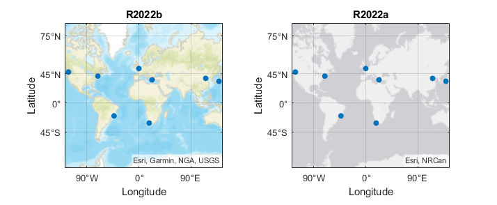
This change does not affect existing code that sets the hold state to "on" between commands.

To reset the basemap when you add a new plot, use the cla reset syntax of the cla function before you create the plot. For example, to update the preceding code, use cla reset between the calls to geobasemap and geoscatter.

lat = [35 -22 51 39 37 42 47 -33];
lon = [139 -43 0 116 23 -71 -122 18];
 
figure
geobasemap streets
cla reset
geoscatter(lat,lon,"filled")

Alternatively, you can change the basemap to the default streets-light by using the geobasemap function. For more information about changing the basemap of geographic axes, see Access Basemaps for Geographic Axes and Charts.