bvpinit

Form initial guess for boundary value problem solver

Syntax

solinit = bvpinit(x,yinit)

solinit = bvpinit(sol,[anew bnew])

solinit = bvpinit(___,parameters)

Description

solinit = bvpinit(x,yinit) uses the initial mesh x and initial solution guess yinit to form an initial guess of the solution for a boundary value problem. You then can use the initial guess solinit as one of the inputs to bvp4c or bvp5c to solve the boundary value problem.

solinit = bvpinit(sol,[anew bnew]) forms an initial guess for the solution on the interval [anew bnew], where sol is a solution structure obtained from bvp4c or bvp5c. The new interval [anew bnew] must be larger than the previous interval on which sol is defined. The previous solution sol is extrapolated to the new interval.

solinit = bvpinit(___,parameters) specifies a vector of initial guesses for parameters with unknown values in the boundary value problem. You can use this syntax with either of the previous input argument combinations.

Examples

Initial Guess of BVP Solution

Create an initial guess of the solution to a BVP, solve the BVP with bvp4c, and then extend the solution to a new domain.

Forming a good initial guess of the solution to a BVP problem is perhaps the most difficult part of solving the problem. BVP solutions are not necessarily unique, so the initial guess can be the deciding factor in which of many solutions the solver returns. The initial guess should satisfy the boundary conditions, and the behavior inbetween should reflect your general expectations about the problem (whether the solution oscillates, is a simple linear function, and so on...).

Consider the differential equation

$${{\mathit{y}}^{\prime }}^{\prime }=-\mathit{y}$$.

The equation is subject to the boundary conditions

$\mathit{y}\left(0\right)=\mathit{y}\left(\pi \right)=0$.

The function that encodes the equation as a first-order system is

function dydx = bvpfun(x,y)
dydx = [y(2)
       -y(1)];
end

Similarly, the function that encodes the boundary conditions is

function res = bcfun(ya,yb)
res = [ya(1)
       yb(1)];
end

You either can include the required functions as local functions at the end of a file (as done here), or you can save them as separate, named files in a directory on the MATLAB® path.

Initial Guess with Function Handle

You reasonably can expect the solution to the equation to be oscillatory, so sine and cosine functions are a good initial guess of the behavior of the solution and its derivative between the fixed boundary points.

function y = guess(x)
y = [sin(x)
     cos(x)];
end

Create a solution structure using 10 equally spaced mesh points in the domain $\left[0,\pi \right]$ and the initial guess function.

xmesh = linspace(0,pi,10);
solinit = bvpinit(xmesh,@guess);

Solve BVP

Call bvp4c with the ode function, boundary conditions, and solution guess. Plot the result.

sol = bvp4c(@bvpfun, @bcfun, solinit);
plot(sol.x,sol.y,'-o')

Local Functions

Listed here are the local helper functions that the BVP solver bvp4c calls to calculate the solution. Alternatively, you can save these functions as their own files in a directory on the MATLAB path.

function dydx = bvpfun(x,y) % equation being solved
dydx = [y(2)
       -y(1)];
end
%-------------------------------------------
function res = bcfun(ya,yb) % boundary conditions
res = [ya(1)
       yb(1)];
end
%-------------------------------------------
function y = guess(x) % guess at solution behavior
y = [sin(x)
     cos(x)];
end
%-------------------------------------------

Extend BVP Solution with Extrapolation

Solve a BVP over an initial interval, and then iteratively extend the interval using each solution as the initial guess for the next interval.

Consider the equation

${{\mathit{y}}^{\prime }}^{\prime }=\mathit{y}$.

As a first-order system, the equation becomes a system of two equations

${{\mathit{y}}_1}^{\prime }={\mathit{y}}_2$,

${{\mathit{y}}_2}^{\prime }={\mathit{y}}_1$.

The equation is initially defined on the interval $\left[0,3\right]$ and is subject to the boundary conditions

$\mathit{y}\left(0\right)=0$,

$\mathit{y}\left(3\right)=1$.

The function that encodes the equation as a first-order system is

function dydx = bvpfun(x,y)
dydx = [y(2)
        y(1)];
end

Similarly, the function that encodes the boundary conditions is

function res = bcfun(ya,yb)
res = [ya(1)
       yb(1)-1];
end

You either can include the required functions as local functions at the end of a file (as done here), or you can save them as separate, named files in a directory on the MATLAB path.

Initial Guess

Use an exponential function as the initial guess for the solution. Since the equation has two solution components, write an initial guess function of the form y = guess(x) that returns a vector.

function y = guess(x)
y = [exp(x)
     exp(x)];
end

A mesh of five points is sufficient to capture the behavior of the guess function.

xmesh = linspace(0,3,5);
solinit = bvpinit(xmesh,@guess);

Solve Equation

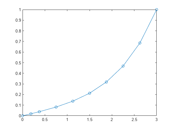
Solve the equation in the initial interval $\left[0,3\right]$ and plot the results for ${\mathit{y}}_1$.

sol = bvp4c(@bvpfun, @bcfun, solinit);
plot(sol.x(1,:),sol.y(1,:),'-o')

Extend Interval

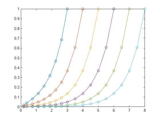
Now, use bvpinit to extend the interval of integration in a loop, solving and plotting each new problem. In each iteration, form the initial guess using the previous solution sol extrapolated to the new interval [0 k]. In each new problem, bvp4c enforces the boundary conditions at the new boundaries [0 k].

hold on
for k = 4:8
    solinit = bvpinit(sol,[0 k]);
    sol = bvp4c(@bvpfun, @bcfun, solinit);
    plot(sol.x(1,:),sol.y(1,:),'-o')
end

This example shows a simplified version of continuation, a useful technique to solve BVPs by breaking the problem down into smaller intervals or simpler problems. For more examples of this technique, see:

• Solve BVP Using Continuation

• Verify BVP Consistency Using Continuation

Local Functions

Listed here are the local helper functions that the BVP solver bvp4c calls to calculate the solution. Alternatively, you can save these functions as their own files in a directory on the MATLAB path.

function dydx = bvpfun(x,y) % equation being solved
dydx = [y(2)
        y(1)];
end
%-------------------------------------------
function res = bcfun(ya,yb) % boundary conditions
res = [ya(1)
       yb(1)-1];
end
%-------------------------------------------
function y = guess(x) % guess at solution behavior
y = [exp(x)
     exp(x)];
end
%-------------------------------------------

Input Arguments

x — Initial mesh

vector

Initial mesh, specified as a vector. To solve the problem on the interval [a,b], specify x(1) as a and x(end) as b. The entries of x must be in increasing order (if a < b) or decreasing order (if a > b). The solver adapts this mesh to the solution (by adding, removing, and moving the mesh points), so a guess like x = linspace(a,b,10) often suffices. To handle difficult problems, place some mesh points where the solution changes rapidly.

• For two-point boundary value problems, the entries of x must be unique. That is, if a < b, the entries must satisfy x(1) < x(2) < ... < x(end). If a > b, the entries must satisfy x(1) > x(2) > ... > x(end).

• For multipoint boundary value problems, you can specify the points in [a,b] at which the boundary conditions apply, other than the endpoints a and b, by repeating their entries in x. For example, consider the vector

  x = [0 0.5 1 1 1.5 2];

  For this mesh, the boundary conditions apply at three points: the endpoints 0 and 2, and the repeated entry 1. In general, repeated entries represent boundary points between regions in [a,b]. The repeated entry 1 divides the interval [0 2] into two regions: [0 1] and [1 2].

Example: solinit = bvpinit(linspace(a,b,10),yinit)

Data Types: single | double | int8 | int16 | int32 | int64 | uint8 | uint16 | uint32 | uint64 | logical
Complex Number Support: Yes

yinit — Initial guess of solution

vector | function

Initial guess of solution, specified as a vector or a function.

• Vector – For each component of the solution, bvpinit replicates the corresponding element of the vector as a constant guess across all mesh points. That is, yinit(i) is a constant guess for the ith component yinit(i,:) of the solution at all the mesh points in x.

• Function – For a given mesh point, the guess function must return a vector whose elements are guesses for the corresponding components of the solution. The function must be of the form

  y = guess(x)

  x is a mesh point and y is a vector whose length is the same as the number of components in the solution. For example, if yinit is a function, then at each mesh point bvpinit calls

  y(:,j) = guess(x(j))

  For multipoint boundary value problems, the guess function must be of the form

  y = guess(x,k)

  y is an initial guess for the solution at x in region k. The function must accept the input argument k, which is provided for flexibility in writing the guess function. However, the function is not required to use k.

Example: solinit = bvpinit(x,[sqrt(3)/2; 0])

Example: solinit = bvpinit(x,@guess)

Data Types: single | double | int8 | int16 | int32 | int64 | uint8 | uint16 | uint32 | uint64 | logical | char | function_handle
Complex Number Support: Yes

parameters — Initial guess for unknown parameter values

scalar | vector

Initial guess for unknown parameter values, specified as a scalar or vector.

Example: solinit = bvpinit(x, yinit, [0 1 sqrt(2)]) specifies a vector of guesses for three unknown parameters.

Example: Type edit mat4bvp to see an example of a BVP with an unknown parameter.

Data Types: single | double | int8 | int16 | int32 | int64 | uint8 | uint16 | uint32 | uint64 | logical
Complex Number Support: Yes

sol — Prior solution

structure

Prior solution, specified as a solution structure returned by bvp4c or bvp5c. If sol contains parameters, they are copied to solinit.

Data Types: struct

Output Arguments

solinit — Initial guess of solution

structure

Initial guess of solution, returned as a structure. Use this structure as the third input to bvp4c or bvp5c to solve the boundary value problem.

Extended Capabilities

Thread-Based Environment

Run code in the background using MATLAB® backgroundPool or accelerate code with Parallel Computing Toolbox™ ThreadPool.

This function fully supports thread-based environments. For more information, see Run MATLAB Functions in Thread-Based Environment.

Version History

Introduced before R2006a