Graph Plotting and Customization
This example shows how to plot graphs, and then customize the display to add labels or highlighting to the graph nodes and edges.
Graph Plotting Objects
Use the plot function to plot graph and digraph objects. By default, plot examines the size and type of graph to determine which layout to use. The resulting figure window contains no axes tick marks. However, if you specify the (x,y) coordinates of the nodes with the XData, YData, or ZData name-value pairs, then the figure includes axes ticks.
Node labels are included automatically in plots of graphs that have 100 or fewer nodes. The node labels use the node names if available; otherwise, the labels are numeric node indices.
For example, create a graph using the buckyball adjacency matrix, and then plot the graph using all of the default options. If you call plot and specify an output argument, then the function returns a handle to a GraphPlot object. Subsequently, you can use this object to adjust properties of the plot. For example, you can change the color or style of the edges, the size and color of the nodes, and so on.
G = graph(bucky);
p = plot(G)
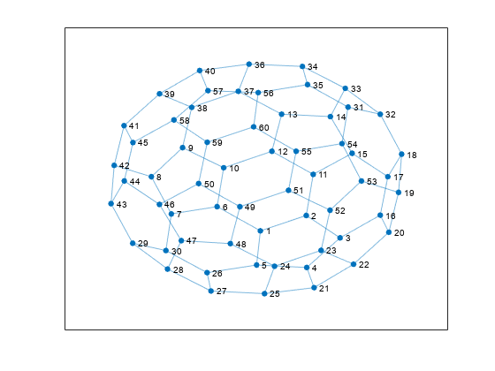
p =
  GraphPlot with properties:

     NodeColor: [0.0660 0.4430 0.7450]
    MarkerSize: 4
        Marker: 'o'
     EdgeColor: [0.0660 0.4430 0.7450]
     LineWidth: 0.5000
     LineStyle: '-'
     NodeLabel: {1×60 cell}
     EdgeLabel: {}
         XData: [0.1033 1.3374 2.2460 1.3509 0.0019 -1.0591 -2.2901 -2.8275 -1.9881 -0.8836 1.5240 0.4128 0.6749 1.9866 2.5705 3.3263 3.5310 3.9022 3.8191 3.5570 1.5481 2.6091 1.7355 0.4849 0.2159 -1.3293 -1.2235 -2.3934 -3.3302 -2.4370 … ] (1×60 double)
         YData: [-1.8039 -1.2709 -2.0484 -3.0776 -2.9916 -0.9642 -1.2170 0.0739 1.0849 0.3856 0.1564 0.9579 2.2450 2.1623 0.8879 -1.2600 0.0757 0.8580 -0.4702 -1.8545 -3.7775 -2.9634 -2.4820 -3.0334 -3.9854 -3.2572 -3.8936 -3.1331 … ] (1×60 double)
         ZData: [0 0 0 0 0 0 0 0 0 0 0 0 0 0 0 0 0 0 0 0 0 0 0 0 0 0 0 0 0 0 0 0 0 0 0 0 0 0 0 0 0 0 0 0 0 0 0 0 0 0 0 0 0 0 0 0 0 0 0 0]

  Show all properties
After you have a handle to the GraphPlot object, use dot indexing to access or change the property values. For a complete list of the properties that you can adjust, see GraphPlot Properties.
Change the value of NodeColor to 'red'.
p.NodeColor = 'red';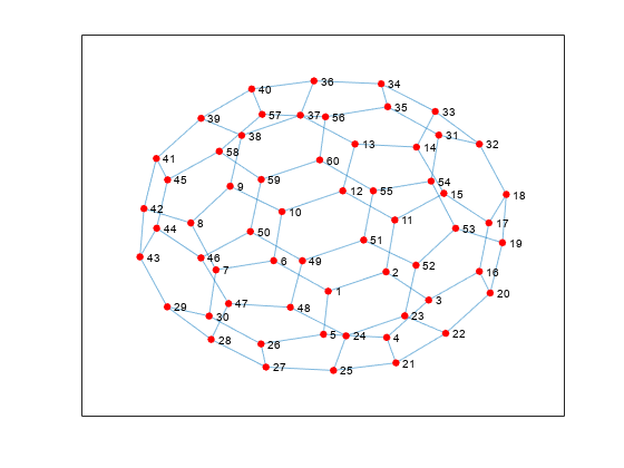
Determine the line width of the edges.
p.LineWidth
ans =
0.5000
Create and Plot Graph
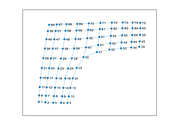
Create and plot a graph representing an L-shaped membrane constructed from a square grid with a side of 12 nodes. Specify an output argument with plot to return a handle to the GraphPlot object.
n = 12;
A = delsq(numgrid('L',n));
G = graph(A,'omitselfloops')
G =
  graph with properties:

    Edges: [130×2 table]
    Nodes: [75×0 table]
p = plot(G)
p =
  GraphPlot with properties:

     NodeColor: [0.0660 0.4430 0.7450]
    MarkerSize: 4
        Marker: 'o'
     EdgeColor: [0.0660 0.4430 0.7450]
     LineWidth: 0.5000
     LineStyle: '-'
     NodeLabel: {1×75 cell}
     EdgeLabel: {}
         XData: [-2.5225 -2.1251 -1.6498 -1.1759 -0.7827 -2.5017 -2.0929 -1.6027 -1.1131 -0.7069 -2.4678 -2.0495 -1.5430 -1.0351 -0.6142 -2.4152 -1.9850 -1.4576 -0.9223 -0.4717 -2.3401 -1.8927 -1.3355 -0.7509 -0.2292 -2.2479 -1.7828 … ] (1×75 double)
         YData: [-3.5040 -3.5417 -3.5684 -3.5799 -3.5791 -3.0286 -3.0574 -3.0811 -3.0940 -3.0997 -2.4191 -2.4414 -2.4623 -2.4757 -2.4811 -1.7384 -1.7570 -1.7762 -1.7860 -1.7781 -1.0225 -1.0384 -1.0553 -1.0568 -1.0144 -0.2977 -0.3097 … ] (1×75 double)
         ZData: [0 0 0 0 0 0 0 0 0 0 0 0 0 0 0 0 0 0 0 0 0 0 0 0 0 0 0 0 0 0 0 0 0 0 0 0 0 0 0 0 0 0 0 0 0 0 0 0 0 0 0 0 0 0 0 0 0 0 0 0 0 0 0 0 0 0 0 0 0 0 0 0 0 0 0]

  Show all properties
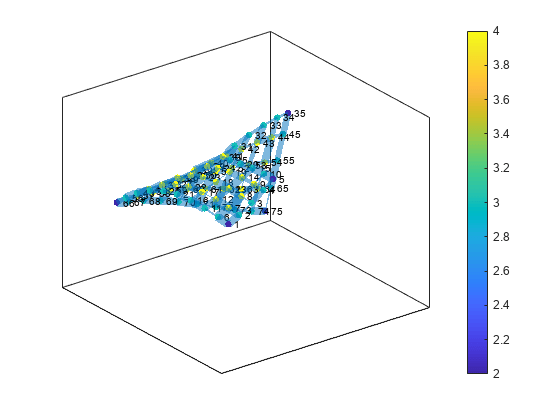
Change Graph Node Layout
Use the layout function to change the layout of the graph nodes in the plot. The different layout options automatically compute node coordinates for the plot. Alternatively, you can specify your own node coordinates with the XData, YData, and ZData properties of the GraphPlot object.
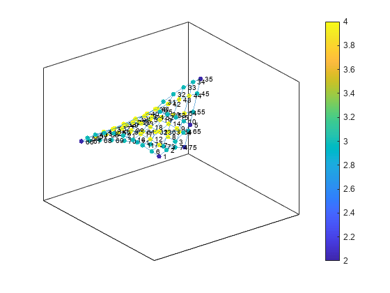
Instead of using the default 2-D layout method, use layout to specify the 'force3' layout, which is a 3-D force directed layout.
layout(p,'force3')
view(3)
Proportional Node Coloring
Color the graph nodes based on their degree. In this graph, all of the interior nodes have the same maximum degree of 4, nodes along the boundary of the graph have a degree of 3, and the corner nodes have the smallest degree of 2. Store this node coloring data as the variable NodeColors in G.Nodes.
G.Nodes.NodeColors = degree(G);
p.NodeCData = G.Nodes.NodeColors;
colorbar
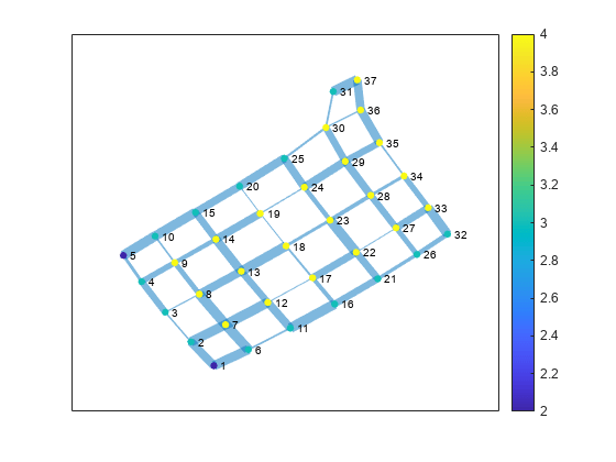
Edge Line Width by Weight
Add some random integer weights to the graph edges, and then plot the edges such that their line width is proportional to their weight. Since an edge line width approximately greater than 7 starts to become cumbersome, scale the line widths such that the edge with the greatest weight has a line width of 7. Store this edge width data as the variable LWidths in G.Edges.
G.Edges.Weight = randi([10 250],130,1);
G.Edges.LWidths = 7*G.Edges.Weight/max(G.Edges.Weight);
p.LineWidth = G.Edges.LWidths;
Extract Subgraph
Extract and plot the top right corner of G as a subgraph, to make it easier to read the details on the graph. The new graph, H, inherits the NodeColors and LWidths variables from G, so that recreating the previous plot customizations is straightforward. However, the nodes in H are renumbered to account for the new number of nodes in the graph.
H = subgraph(G,[1:31 36:41]);
p1 = plot(H,'NodeCData',H.Nodes.NodeColors,'LineWidth',H.Edges.LWidths);
colorbar
Label Nodes and Edges
Use labeledge to label the edges whose width is larger than 6 with the label, 'Large'. The labelnode function works in a similar manner for labeling nodes.
labeledge(p1,find(H.Edges.LWidths > 6),'Large')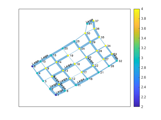
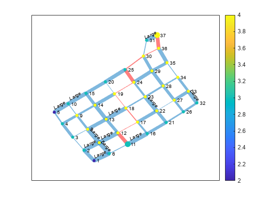
Highlight Shortest Path
Find the shortest path between node 11 and node 37 in the subgraph, H. Highlight the edges along this path in red, and increase the size of the end nodes on the path.
path = shortestpath(H,11,37)
path = 1×10

    11    12    17    18    19    24    25    30    36    37
highlight(p1,[11 37])
highlight(p1,path,'EdgeColor','r')
Remove the node labels and colorbar, and make all of the nodes black.
p1.NodeLabel = {};
colorbar off
p1.NodeColor = 'black';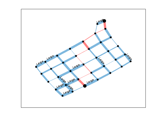
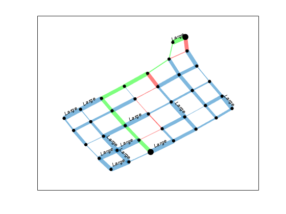
Find a different shortest path that ignores the edge weights. Highlight this path in green.
path2 = shortestpath(H,11,37,'Method','unweighted')
path2 = 1×10

    11    12    13    14    15    20    25    30    31    37
highlight(p1,path2,'EdgeColor','g')
Plotting Large Graphs
It is common to create graphs that have hundreds of thousands, or even millions, of nodes and/or edges. For this reason, plot treats large graphs slightly differently to maintain readability and performance. The plot function makes these adjustments when working with graphs that have more than 100 nodes:
The default graph layout method is always
'subspace'.The nodes are no longer labeled automatically.
The
MarkerSizeproperty is set to2. (Smaller graphs have a marker size of4).The
ArrowSizeproperty of directed graphs is set to4. (Smaller directed graphs use an arrow size of7).
See Also
graph | digraph | plot | layoutcoords | GraphPlot