Main Content

mapprofile

Interpolate between waypoints on terrain

    Description

    Use Unit Sphere and Get Range in Degrees

    [zq,distq,latq,lonq] = mapprofile(Z,R,lat,lon) interpolates intermediate points between the waypoints specified by lat and lon. You must specify the elevation data Z and spatial reference R for the terrain. For each intermediate point, the function returns the interpolated terrain height in zq, the distance from the first waypoint (the range) in distq, the latitude in latq, and the longitude in lonq.

    Specify Range Units

    example

    [zq,distq,latq,lonq] = mapprofile(Z,R,lat,lon,units) specifies the units units for distq. The function calculates surface distances using the default radius of the Earth (equivalent to 6371 kilometers).

    [zq,distq,latq,lonq] = mapprofile(Z,R,lat,lon,units,trackmethod) additionally specifies whether intermediate points are along great circles or rhumb lines.

    example

    [zq,distq,latq,lonq] = mapprofile(Z,R,lat,lon,units,trackmethod,interpmethod) additionally specifies the interpolation method.

    Specify Reference Ellipsoid

    [zq,distq,latq,lonq] = mapprofile(Z,R,lat,lon,ellipsoid) specifies the reference ellipsoid for the coordinates. This syntax returns distq using the units of the semimajor axis of the reference ellipsoid.

    [zq,distq,latq,lonq] = mapprofile(Z,R,lat,lon,ellipsoid,trackmethod) additionally specifies whether intermediate points are along great circle tracks or rhumb line tracks.

    [zq,distq,latq,lonq] = mapprofile(Z,R,lat,lon,ellipsoid,trackmethod,interpmethod) additionally specifies the interpolation method.

    Display and Interactively Select Coordinates

    mapprofile(___) displays an elevation profile of the intermediate points in a new figure on an axesm-based map.

    example

    [___] = mapprofile enables you to interactively select waypoints on the current axesm-based map. If the current object on the map is a regular data grid, then the function uses the z-coordinate data (the ZData property) as the terrain elevation data. Otherwise, the function uses z-coordinate data from the first regular data grid it finds on the map. If the grid does not have z-coordinate data, then the function uses the color data (the CData property), instead. To finish selecting points, press Enter.

    Examples

    collapse all

    Load elevation data and a geographic cells reference object for the Korean peninsula. Compute the elevation profile between two points in the region, specifying the units for the range (distq) as kilometers. By default, the mapprofile function uses bilinear interpolation along a great circle track.

    load korea5c
    
    lat = [40.5 30.7];
    lon = [121.5 133.5];
    [zq,distq,latq,lonq] = mapprofile(korea5c,korea5cR,lat,lon,"km");

    Plot the track over a satellite basemap.

    figure
    geolimits(korea5cR.LatitudeLimits,korea5cR.LongitudeLimits)
    hold on
    geoplot(latq,lonq,"w","LineWidth",2)
    geobasemap satellite

    Figure contains an axes object. The axes object contains an object of type line.

    Display the elevation profile on a Cartesian plot.

    figure
    plot(distq,zq)
    xlabel("Range (kilometers)")
    ylabel("Elevation (meters)")

    Figure contains an axes object. The axes object contains an object of type line.

    Load world topography data into the workspace as an array and a geographic raster reference object. Calculate an elevation profile for the great circle track between San Francisco and New York City, using nearest neighbor interpolation.

    load topo60c
    
    lat = [37.77 40.71];
    lon = [-122.41 -74.01];
    [zqgc,distqgc,latqgc,lonqgc] = mapprofile(topo60c,topo60cR,lat,lon,"km","gc","nearest");

    Calculate an elevation profile for the rhumb line track between the same cities, using bicubic interpolation.

    [zqrh,distqrh,latqrh,lonqrh] = mapprofile(topo60c,topo60cR,lat,lon,"km","rh","bicubic");

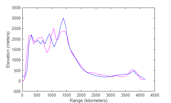
    Display both tracks on a map. Use magenta for the great circle track and blue for the rhumb line track.

    figure
    geoplot(latqgc,lonqgc,"m","LineWidth",1.5)
    hold on
    geoplot(latqrh,lonqrh,"b","LineWidth",1.5)
    geobasemap streets

    Display both elevation profiles on a Cartesian plot.

    figure
    plot(distqgc,zqgc,"m")
    hold on
    plot(distqrh,zqrh,"b")
    xlabel("Range (kilometers)")
    ylabel("Elevation (meters)")

    Load terrain elevation data for the Korean peninsula into the workspace as an array and a geographic cells reference object. Specify the coordinates of four waypoints.

    load korea5c
    lat = [43 43 41 38];
    lon = [116 120 126 128];

    Display the elevation profile on a map by omitting the output arguments. When you specify more than two waypoints, the function displays the result in 3-D.

    mapprofile(korea5c,korea5cR,lat,lon)

    Add coastlines and city locations to the map.

    load coastlines
    plotm(coastlat,coastlon)
    geoshow("worldcities.shp","Marker",".","Color","r")

    Input Arguments

    collapse all

    Elevation data grid, specified as an m-by-n array.

    Data Types: single | double

    Spatial reference for Z, specified as a GeographicCellsReference or GeographicPostingsReference object. The RasterSize property of R must be consistent with size(Z).

    Latitude coordinates of the waypoints, in degrees, specified as a vector. You can separate sets of waypoints into line sequences using NaN values. The NaN values in lat must correspond to the NaN values in lon.

    The size of lat must match the size of lon.

    Data Types: single | double

    Longitude coordinates of the waypoints, in degrees, specified as a vector. You can separate sets of waypoints into line sequences using NaN values. The NaN values in lon must correspond to the NaN values in lat.

    The size of lat must match the size of lon.

    Data Types: single | double

    Units for distq, specified as one of these options:

    • These angular units.

      ValueUnit Name
      "degree", "degrees", "deg"Degrees
      "radian", "radians", "rad"Radians
    • Any length unit supported by the validateLengthUnit function.

      ValueUnit Name
      "m", "meter", "meters", "metre", "metres"Meters
      "cm", "centimeter", "centimeters", "centimetre", "centimetres"Centimeters
      "mm", "millimeter", "millimeters", "millimetre", "millimetres"Millimeters
      "micron", "microns"Microns
      "km", "kilometer", "kilometers", "kilometre", "kilometers"Kilometers
      "nm", "naut mi", "nautical mile", "nautical miles"Nautical miles
      "ft", "international ft", "foot", "international foot", "feet", "international feet"Feet
      "in", "inch", "inches"Inches
      "yd", "yds", "yard", "yards"Yards
      "mi", "mile", "miles", "international mile", "international miles"Miles
      "sf", "survey ft", "US survey ft", "U.S. survey ft", "survey foot", "US survey foot", "U.S. survey foot", "survey feet", "US survey feet", "U.S. survey feet"U.S. survey feet
      "sm", "survey mile", "survey miles", "statute mile", "statute miles", "US survey mile", "US survey miles", "U.S. survey mile(s)", "U.S. survey miles"U.S. survey miles (statute miles)
      "Clarke's foot", "Clarkes foot"Clarke's feet
      "German legal metre", "German legal meter"German legal metres
      "Indian foot"Indian feet

    This argument is case insensitive.

    Data Types: char | string

    Reference ellipsoid, specified as a referenceSphere object, a referenceEllipsoid object, an oblateSpheroid object, or a two-element vector of the form [semimajor_axis eccentricity], where semimajor_axis is the length of the semimajor axis and eccentricity is the eccentricity. The values semimajor_axis and eccentricity must be of data type double.

    The default value of [1 0] represents the unit sphere.

    When you specify the ellipsoid argument, the mapprofile function returns distq in the units of the semimajor axis of the reference ellipsoid.

    If you do not specify the ellipsoid argument and R contains a geocrs object in its GeographicCRS property, then the mapprofile function uses the ellipsoid contained in the geocrs object. For example, given a reference object R, the function uses R.GeographicCRS.Spheroid.

    Track method, specified as one of these options:

    • "rh" — Find track points along rhumb line paths.

    • "gc" — For spheres, find track points along great circle paths. For ellipsoids, find track points along geodesic paths.

    Data Types: char | string

    Interpolation method, specified as one of these options:

    • "bilinear" — Use linear interpolation.

    • "bicubic" — Use cubic interpolation.

    • "nearest" — Use nearest neighbor interpolation.

    Data Types: char | string

    Output Arguments

    collapse all

    Terrain heights of the intermediate points, returned as a numeric vector. The function calculates the terrain heights using the same units as Z.

    The number of intermediate points depends on the density of the terrain elevation data. When you increase the density of the data, the mapprofile function returns more intermediate points.

    The sizes of zq, distq, latq, and lonq match.

    Range, returned as a numeric vector. For each intermediate point, the range is the distance from the first point to the intermediate point. If you separate the input waypoints into sequences using NaN values, then the function calculates the distance of each intermediate waypoint from the first waypoint in the corresponding sequence.

    By default, the units for distq are degrees. You can specify the units for distq using the units or ellipsoid argument.

    The number of intermediate points depends on the density of the terrain elevation data. When you increase the density of the data, the mapprofile function returns more intermediate points.

    The sizes of zq, distq, latq, and lonq match.

    Latitudes of the intermediate points, in degrees, returned as a numeric vector.

    The number of intermediate points depends on the density of the terrain elevation data. When you increase the density of the data, the mapprofile function returns more intermediate points.

    The sizes of zq, distq, latq, and lonq match.

    Longitudes of the intermediate points, in degrees, returned as a numeric vector.

    The number of intermediate points depends on the density of the terrain elevation data. When you increase the density of the data, the mapprofile function returns more intermediate points.

    The sizes of zq, distq, latq, and lonq match.

    Version History

    Introduced before R2006a

    expand all

    See Also

    Functions