Radar Performance Analysis over Terrain
The performance of a radar system is highly dependent on the environment in which it operates. While the free space spreading loss might be such that the target signal-to-noise ratio (SNR) does not satisfy the minimum detectability threshold for the desired probability of detection and probability of false alarm, the detectability of a target might further suffer in some terrains as there might be no direct, unobstructed line-of-sight from the radar to the target. As you will see in this example, as the elevation of a target increases above the terrain, the radar has a better chance of detecting the target.
In this example, you will learn how to analyze the performance of a ground-based, long-range terminal airport surveillance radar tasked with detecting an aircraft in the presence of heavy, mountainous clutter. The example first defines the radar system operating characteristics and its global position. It then defines the target and its trajectory. Finally, the detectability of the target as it moves through its trajectory is presented along with detailed visualizations.
Define Radar
To start, specify a C-band long-range, terminal airport surveillance radar with the following parameters:
Peak power: 1 kW
Operating frequency: 6 GHz
Transmit and receive antenna: 2 degrees in azimuth, 5 degrees in elevation
Pulse width: 1 μs
rdrppower = 1e3;            % Peak power (W)
fc = 6e9;                   % Operating frequency (Hz)
hpbw = [2; 5];              % Half-power beamwidth [azimuth; elevation] (deg)
rdrpulsew = 1e-6;           % Pulse width (s)
lambda = freq2wavelen(fc);  % Wavelength (m)
Convert the transmitter half-power beamwidth (HPBW) values to gain using the beamwidth2gain function. Assume a cosine rectangular aperture, which is a good approximation for a real-world antenna.
rdrgain = beamwidth2gain(hpbw,"CosineRectangular"); % Transmitter and receiver gain (dB)
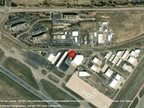
Define the radar ground location as the Rocky Mountain Metropolitan Airport in Broomfield, Colorado, USA. The radar is mounted on a tower 10 meters above the ground. The radar altitude is the sum of the ground elevation and the radar tower height referenced to the mean sea level (MSL).
rdrlat = 39.913756;         % Radar latitude (deg)
rdrlon = -105.118062;       % Radar longitude (deg)
rdrtowerht = 10;            % Antenna height (m)
rdralt = 1717 + rdrtowerht; % Radar altitude (m)
To visualize the radar location, import the relevant terrain data from the United States Geological Survey (USGS). The input height to geoplot3 is referenced to the geoid, or mean sea level.
dtedfile = "n39_w106_3arc_v2.dt1";
attribution = "SRTM 3 arc-second resolution. Data available from the U.S. Geological Survey.";
[Zterrain,Rterrain] = readgeoraster(dtedfile,"OutputType","double");

% Visualize the location using the geographic globe plot.
addCustomTerrain("southboulder",dtedfile,Attribution=attribution);
fig = uifigure;
g = geoglobe(fig,Terrain="southboulder");
hold(g,"on")
h_rdrtraj = geoplot3(g,rdrlat,rdrlon,rdralt,"ro",LineWidth=6,MarkerSize=10);

Note that the limits for the file correspond to the region around Boulder, Colorado, USA, and the resolution corresponds to DTED level-1, which has a sample resolution of 3 arc seconds or about 90 meters.
Define Target
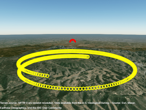
Consider a large commercial aircraft as the target. Assume the aircraft trajectory is a corkscrew maneuver, where the aircraft descends rapidly in a spiral.
tlat0 = 39.80384;           % Target initial latitude (deg)
tlon0 = -105.49916;         % Target initial longitude (deg)
tht0 = 3000;                % Target initial height (m)
azs = 1:2:540;              % Target azimuth (deg)
r = 5000;                   % Target slant range (m)

% Convert from polar coordinates to Cartesian East, North, Up (ENU).
[X,Y] = pol2cart(deg2rad(azs),r);

% Convert ENU to geodetic.
Z = linspace(0,1000,numel(azs));
wgs84 = wgs84Ellipsoid;
[tlat,tlon,tht] = enu2geodetic(X,Y,Z,tlat0,tlon0,tht0,wgs84);

% Define the target altitude relative to the geoid.
talt = tht - egm96geoid(tlat,tlon); % Target altitude (m)
For simplicity, assume the waypoints are obtained at a constant sampling rate of 0.1 Hz. The trajectory can be generated using geoTrajectory with positions specified as latitude, longitude, and height. Height for geoTrajectory is referenced to the WGS84 ellipsoid.
fs = 0.1;
t = (0:length(X)-1)/fs;
ttraj = geoTrajectory([tlat.' tlon.' tht.'],t,SampleRate=fs);
Plot the ground truth trajectory over the terrain.
h_ttraj = geoplot3(g,tlat,tlon,talt,"yo",LineWidth=3);
campos(g,39.77114,-105.62662,6670)
camheading(g,70)
campitch(g,-12)
The radar cross section (RCS) for an aircraft is typically from 1 to 10 square meters. For this example, consider the aircraft as an isotropic point target with an RCS of 10 square meters.
trcs = pow2db(10); % Target RCS (dBsm)Simulate the Scenario
Now that the radar and target have been defined, build the scenario, which is composed of a terminal airport radar and large commercial aircraft in the presence of mountainous clutter. Run the simulated scenario for the duration of the aircraft trajectory.
scene = radarScenario(IsEarthCentered=true,UpdateRate=fs,StopTime=t(end));
rdrplatform = platform(scene,Position=[rdrlat,rdrlon,rdralt],Sensor=radarDataGenerator);
tplatform = platform(scene,Trajectory=ttraj,Signatures= ...
    {rcsSignature(Azimuth=[-180 180],Elevation=[-90 90],Pattern=trcs)});
The line-of-sight path from the radar to the target is determined for each point in the target trajectory. For locations where the aircraft is not occluded by the terrain, an SNR value is calculated using the radar equation, including the propagation factor along the path.
The propagation factor is calculated using the radarpropfactor function. The default permittivity model in radarpropfactor is based on a sea permittivity model in Blake's Machine Plotting of Radar Vertical-Plane Coverage Diagrams. Such a model is not applicable in this example. Thus, the first step in simulating more realistic propagation is to select a more appropriate permittivity. Use the earthSurfacePermittivity function with the vegetation flag. Assume an ambient temperature of 21.1 degrees Celsius, which is about 70 degrees Fahrenheit. Assume a gravimetric water content of 0.3.
temp = 21.1;                % Ambient temperature (degrees Celsius)
gwc = 0.3;                  % Gravimetric water content
[~,~,epsc] = earthSurfacePermittivity("vegetation",fc,temp,gwc);
Calculate the propagation factor using the radarpropfactor function. Include the following in the calculation:
Surface permittivity
Standard deviation of height along the path
Elevation beamwidth
tsnr = -inf(size(t));
F = zeros(size(t));
trange = zeros(size(t));
isVisible = false(size(t));
idx = 1;

while advance(scene)
    tpose = pose(tplatform,CoordinateSystem="Geodetic");
    tpos = tpose.Position;
    [isVisible(idx),~,~,h] = los2(Zterrain,Rterrain,rdrlat,rdrlon, ...
        tpos(1),tpos(2),rdralt,tpos(3),"MSL","MSL");
    hgtStdDev = std(h);
    if isVisible(idx)
        trange(idx) = llarangeangle([rdrlat rdrlon rdralt],tpos,1);
        F(idx) = radarpropfactor(trange(idx),fc,rdralt,tpos(3), ...
            SurfaceRelativePermittivity=epsc,...
            SurfaceHeightStandardDeviation=hgtStdDev, ...
            ElevationBeamwidth=hpbw(2));
    end
    idx = idx+1;
end
Calculate the SNR along the trajectory.
tsnr(isVisible) = radareqsnr(lambda,trange(isVisible).',rdrppower,rdrpulsew,...
    RCS=trcs,Gain=rdrgain,PropagationFactor=F(isVisible).');
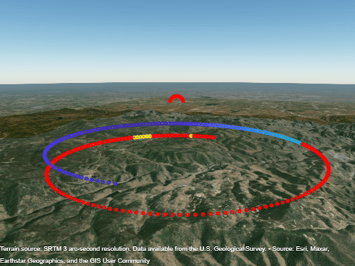
Next, plot the SNR along the trajectory.
tsnr_finiteidx = ~isinf(tsnr);
tsnr_cidx = zeros(size(tsnr));
cmap = colormap(g);
numclvls = size(cmap,1);
tsnr_cidx(tsnr_finiteidx) = discretize(tsnr(tsnr_finiteidx),numclvls-1);
tsnr_cidx(~tsnr_finiteidx) = numclvls;

delete(h_ttraj);
hsnr = zeros(size(tsnr));
for m = 1:numel(tsnr)
    hsnr(m) = geoplot3(g,tlat(m),tlon(m),talt(m), ...
        Marker="o",LineWidth=2,MarkerSize=1);
    if tsnr_finiteidx(m)
        set(hsnr(m),"Color",cmap(tsnr_cidx(m),:));
    else
        set(hsnr(m),"Color","r");
    end
end

As the aircraft performs the corkscrew maneuver, the SNR of the received signal might vary, as shown in the figure. The radar has an unobstructed view of the aircraft if there is a line-of-sight path. The red portion of the trajectory indicates that there is no line-of-sight path between the aircraft and the radar.
For the surveillance radar, the desired performance index is a probability of detection (Pd) of 0.9 and probability of false alarm (Pfa) below 1e-6. To make the radar system design more feasible, you can use a pulse integration technique to reduce the required SNR. For this system, assume noncoherent integration of 32 pulses. A good approximation of the minimum SNR needed for a detection at the specified Pd and Pfa can be computed by the detectability function.
pd = 0.9;
pfa = 1e-6;
minsnr_32p = detectability(pd,pfa,32);
isdetectable_32p = tsnr >= minsnr_32p;
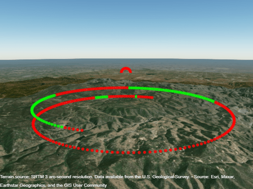
Observe in which part of the trajectory the target is detectable (shown in green) given the minimum SNR requirement. Note that the existence of a line-of-sight link does not guarantee that the target is detectable.
for m = 1:numel(tsnr)
    if isdetectable_32p(m)
        set(hsnr(m),Color="g");
    else
        set(hsnr(m),Color="r");
    end
end

To improve detectability with surveillance radars, often radar engineers discuss maximizing the power-aperture product of the system. This generally translates to increasing the physical size or peak power of a system. It can also be considered in terms of illumination time (i.e., energy on target). Some methods to improve detectability include:
Increasing the peak power: This can be difficult to achieve due to limitations on the power supply and on the radar platform location. Furthermore, if there is a requirement for low probability of intercept (LPI), increasing peak power is often undesirable.
Increasing the physical size of the antenna aperture: Increasing the physical size of the antenna results in an increase in the associated gain and decrease in the half-power beamwidth. Limitations of the platform or location might make increasing the physical size of the antenna aperture infeasible. Additionally, with a finer beamwidth, it becomes more important that the antenna beam is steered towards the target under test.
Increasing the number of pulses to be integrated: This will bring the detectability to a lower value. However, if the aircraft is maneuvering at a high speed, then it might take too long to collect all of the transmitted pulses under the assumption of target stationarity. If the target stationarity assumption is invalid, additional signal processing steps will need to be taken to mitigate the range walk of the target.
Increasing the average power: Rather than increasing the peak power, one can increase the average power by increasing the duty cycle. Increasing the duty cycle means increasing either the pulse width or the pulse repetition frequency (PRF), which might put undue burden on the radar hardware. The downside to increasing the pulse width is an increase in the minimum range and potentially overlapping, inseparable target returns. On the other hand, increasing the pulse repetition frequency decreases the maximum unambiguous range, which might be undesirable for a long-range surveillance system, especially if it is not performing a disambiguation technique.
The above list, while in no way exhaustive, shows some of the tradeoffs in the design of an terminal airport surveillance system. For this example, increase the peak power. Since this is a ground-based system, increasing the power is not expected to be too burdensome. Additionally, other airport radars like the ASR-9 operate at a peak power of about 1 MW. Since this is an airport radar, there is no need for LPI requirements.
Consider the case where the peak power is increased to 10 kW.
rdrppower = 10e3;          % Peak power (W)

% Recalculate the SNR along the trajectory.
tsnr(isVisible) = radareqsnr(lambda,trange(isVisible).',rdrppower,rdrpulsew,...
    RCS=trcs,Gain=rdrgain,PropagationFactor=F(isVisible).');

% Determine the regions of the trajectory that are now detectable given the
% newly updated SNR.
isdetectable_32p = tsnr >= minsnr_32p;
Notice that by increasing the peak power, the regions at the end of the trajectory that were previously undetected now satisfy the minimum SNR threshold.
for m = 1:numel(tsnr)
    if isdetectable_32p(m)
        set(hsnr(m),Color="g");
    else
        set(hsnr(m),Color="r");
    end
end

Summary
In this example, SNR is calculated and visualized for a ground-based, long-range terminal airport surveillance radar tasked with detecting an aircraft in the presence of heavy, mountainous clutter. The example shows how to calculate the line-of-sight given a target trajectory. It also shows that the existence of a line-of-sight link does not necessarily guarantee that the target is detectable. This example considers some design tradeoffs to improve target detectability, discussing how radar parameters can be modified to match other system requirements. The example can be easily extended for other aircraft, different trajectory sets, and different terrain maps.
% Clean up by closing the geographic globe and removing the imported
% terrain data.
if isvalid(fig)
    close(fig)
end
removeCustomTerrain("southboulder")
See Also
Functions
addCustomTerrain|geoglobe|geoplot3|radarScenario(Radar Toolbox) |radareqsnr(Radar Toolbox)
Topics
- Radar Vertical Coverage over Terrain (Radar Toolbox)